https://www.zcyphygeodesy.com/en/h-nd-147.html
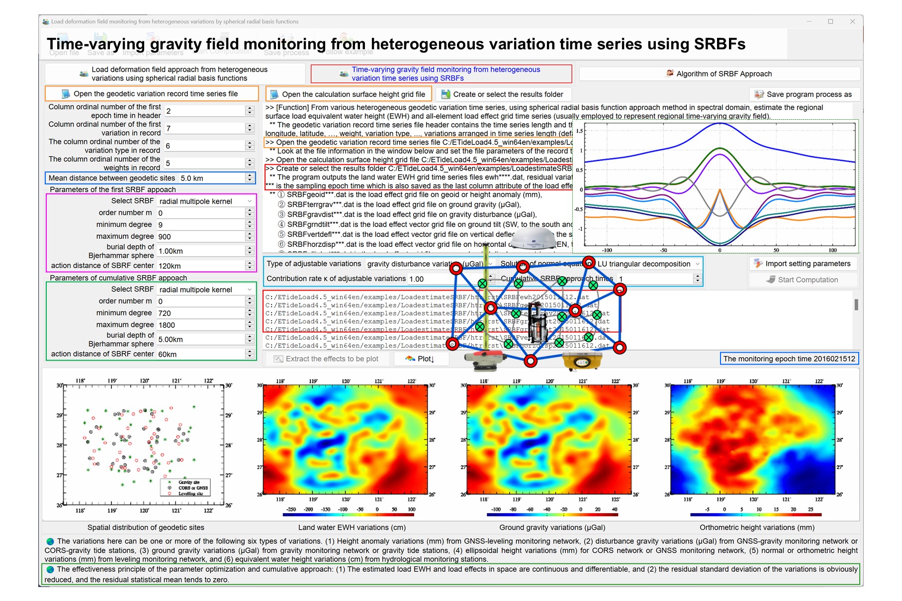
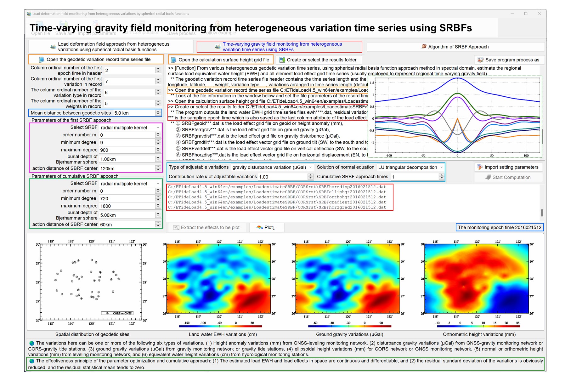
From various heterogeneous geodetic variation time series, using spherical radial basis function approach method in spectral domain, estimate the regional surface load equivalent water height (EWH) and all-element load effect grid time series (usually employed to represent regional time-varying gravity field).
It is technically required that the long wave parts of the load effects on geodetic variations should be removed to satisfy the regional SRBF approach condition.
The variations here can be one or more of the following six types of variations. (1) Height anomaly variations (mm) from GNSS-leveling monitoring network, (2) disturbance gravity variations (μGal) from GNSS-gravity monitoring network or CORS-gravity tide stations, (3) ground gravity variations (μGal) from gravity monitoring network or gravity tide stations, (4) ellipsoidal height variations (mm) for CORS network or GNSS monitoring network, (5) normal or orthometric height variations (mm) from leveling monitoring network, and (6) equivalent water height variations (cm) from hydrological monitoring stations.
The Earth’s Load Love number file love_load_cm.dat from a Regional EIAstic Rebound calculator (REAR1.0, 2015).
LoadeffectSRBFheterovariation.f90
Input parameters: obstmsqdfl - the heterogeneous geodetic variation record time series file name.
The file header contains the time series length and the sampling epoch time arranged with time. Record format: ID (the site name / no), longitude, latitude, …, weight, variation type, …, variations arranged in time series length (default value is 9999.0000).
Variation type = 1 represents the height anomaly variation (mm), = 2 represents gravity disturbance variation (μGal), = 3 represents ground gravity variation (μGal), = 4 represents ground ellipsoidal height variation (mm), = 5 represents normal or orthometric height variation (mm), and = 6 represents equivalent water height variations (cm).
Input parameters: dtmfl - The calculation surface height grid file name.
The calculation surface height is the height of the calculation point relative to the ground surface. When calculating the ground load deformation field, enter the zero-value grid. The calculation surface height grid specification is employed to specify the latitude and longitude range and spatial resolution of the land water EWH grid to be estimated.
The program requires that the grid range of the calculation surface height must be larger than the monitoring site distribution range to absorb the edge effect. The actual effective range of the land water EWH and load effect grid to be estimated will be less than the coverage range of these monitoring sites.
Input parameters: lnth, itern - the mean distance (m) between geodetic sites and cumulative SRBF approach times.
Input parameters: cntrlknd, kwgh  - the type (1~6) of adjustable variation and contribution rate.
Input parameter: knd - the method of the solution of normal equation, knd=1 LU triangular decomposition method, =2 Cholesky decomposition, =3 least square qr decomposition, =4 Minimum norm singular value decomposition.
Input parameters: hepch, frow - the column ordinal number of the first epoch time in header and column ordinal number of the first variation in record.
Input parameters: kndrow, wghrow - the column ordinal number of the variation type and its weight in record.
Input parameters: krbf, krbf1,order,order1 - type and order of the main SRBF and cumulative SRBF1.
Input parameters: dr, dr1, dpth, dpth1 - the action distance (m) of main SRBF center and cumulative SRBF1 center and the two Bjerhammar sphere burial depths.
Input parameters: minN,maxN, minN,1maxN1 - minimum and maximum degree of the main SRBF and cumulative SRBF1 Legendre expansions.
LoadestmateSRBF(dtmfl,obstmsqdfl,flv,dtrow,inp)
Input parameters: flv(:,3) – load love numbers.
Input parameters: dtrow - the column ordinal number of the current variations in the geodetic variation record time series file record.
Output the land water EWH grid file ewh****.dat, residual geodetic variation file rnt***.txt and 10 kinds of load effect grid files in the following.
  SRBFgeoid***.dat is the load effect grid file on geoid or height anomaly (mm).
  SRBFterrgrav***.dat is the load effect grid file on ground gravity (μGal).
  SRBFgravdist***.dat is the load effect grid file on gravity disturbance (μGal).
  SRBFgrndtilt***.dat is the load effect vector grid file on ground tilt (SW, to the south and to the west, mas).
  SRBFvertdefl***.dat is the load effect vector grid file on vertical deflection (SW, to the south and to the west, mas).
  SRBFhorzdisp***.dat is the load effect vector grid file on horizontal displacement (EN, to the east and to the north, mm).
  SRBFelliphgt***.dat is the load effect grid file on ground radial displacement (mm).
  SRBForthohgt***.dat is the load effect grid file on ground normal or orthometric height (mm).
  SRBFgradient***.dat is the load effect grid file on radial gravity gradient (mE).
  SRBFhorzgrad***.dat is the load effect vector grid file on horizontal gravity gradient (NW, to the north and to the west, mE).
Here, *** is the sampling epoch time which is also saved as the last column attribute of the load effect grid file header.
The module also outputs the SRBF spatial curve file SRBFspc.rbf and spectral curve file SRBFdgr.rbf of 11 kinds of geodetic variations into the current directory.
SRBFspc.rbf file header format: SRBF type (0-radial multipole kernel function, 1-Poisson wavelet kernel function), order of SRBF, Minimum and maximum degree of SRBF Legendre expansion, buried depth (km). The record format: spherical distance (km), the normalized SRBF values from the load EWH, height anomaly, ground gravity, gravity disturbance, ground tilt, vertical deflection, horizontal displacement, radial displacement, orthometric height, radial gravity gradient and horizontal gradient variations.
The file header of SRBFdgr.rbf is the same as SRBFspc.rbf. The record format: degree n of SRBF Legendre expansion, the degree-n normalized SRBF values from the load EWH, height anomaly, ground gravity, gravity disturbance, ground tilt, vertical deflection, horizontal displacement, radial displacement, orthometric height, radial gravity gradient and horizontal gradient variations.
ReuterGrid(rhd,lvl,Kt,blat,nn,mm,nln,sr,dl,nrd,lon)
Input parameters: rhd(4) - minimum and maximum longitude, minimum and maximum geocentric latitude of the Reuter network.
Input parameters: lvl, nn, mm - the Reuter network level, maximum number of Reuter centers in the meridian direction and that in the parallel direction.
Return parameter: Blat - the geocentric latitude (degree decimal) of Reuter centers in the first parallel direction.
Return parameters: Kt - the number of Reuter centers, equal to the number of unknowns to be estimated.
Return parameters: nln(nn) - the number of the Reuter centers in the parallel direction.
Return parameters: sr(nn) - the percentage of the difference between the area of the Reuter cell-grid in the parallel direction and the area of the equatorial cell-grid.
Return parameters: dl(nn) - the longitude interval (degree decimal) of the Reuter centers in the parallel direction.
Return parameters: nrd(nn,mm) - ordinal number value of the Reuter centers.
Return parameters: lon(nn,mm) - longitude value of the Reuter centers.
Edgnode(enode,rlatlon,lvl,edgn,lon,blat,nln,gpnt,nn,mm)
The module calculates the number of observation points in the Reuter cell-grid and the number gpnt of Reuter centers corrected.
Return parameter: edgn - the number of Reuter centers around the edge of the Reuter grid.
Return parameters: enode(edgn) - the ordinal number value of Reuter centers in the edge of the Reuter grid.
Return parameter: rlatlon(edgn,2) - the geocentric latitude and longitude (degree decimal) of Reuter centers in the edge of the Reuter grid.
SRBF11all(RBF,flv,order,krbf,mpn,mdp,mp2,minN,maxN,NF,nta)
Return parameters: RBF(NF+1,11) - The SRBF curves of all 11 elements, which is calculated by the action distance of SRBF center and Reuter grid level.
Where RBF(NF+1,knd): knd=1 EWH, =2 height anomaly, =3 ground gravity, =4 gravity disturbance, =5 ground tilt, =6 vertical deflection, =7 horizontal displacement, =8 ground radial displacement, =9 ground normal or orthometric height, =10 radial gravity gradient, =11 horizontal gravity gradient.
Input parameters: flv(:,3) - Load love numbers.
Input parameters: nta - the bandwidth parameter and nta = (r0-dpth)/r0, here dpth is the Bjerhammar sphere burial depth and r0 is the average geocentric distance of observation points.
Input parameters: krbf,order - krbf=0 radial multipole kernel function, =1 Poisson wavelet kernel function and order is the order number of SRBF.
Input parameters: mpn(maxN-minN+1, NF+1), mdp(maxN-minN+1, NF+1), mp2(maxN-minN+1, NF+1) - all minN to maxN degree Legendre functions and their first and second derivatives.
RtGridij(rln,ki,kj,blat,lvl,nn,mm,nln,dl,lon)
Input parameters: rln(3) - the spherical coordinates of the calculation point。
Return parameters: ki,kj - the position of the calculation point rln(3) in the Reuter grid, It is represented by the element of the 2-D ordinal number array of the Reuter grid and ki>0, kj>0.
GNormalfd(BLH,NFD,GRS)
Return parameters: NFD(5) - the normal geopotential (m2/s2), normal gravity (mGal), normal gravity gradient (E), normal gravity line direction (', expressed by its north declination relative to the center of the Earth center of mass) or normal gravity gradient direction (', expressed by its north declination relative to the Earth center of mass).
LegPn_dt2(pn,dp1,dp2,n,t) ! t=cos ψ
EqHestens(BPB,xx,nn,BPL); EqJordon(BPB,xx,nn,BPL)
EqCholesky(BPB,XX,nn,BPL); EqueSVD(BPB,XX,nn,BPL)
RidgeEstimate(BPB,xx,nn,BPL); Equsolve(BPB,xx,nn,BPL,knd,bf)
BLH_RLAT(GRS, BLH, RLAT); LegPn02(mpn,mdp,mp2,minN,maxN,NF,dr)
RBFvalue(RBF(:,1),NF,dr,dln(2),tmp); drln(rln,rlnk,dln)
PickReclong(line, kln, rec, nn); Stat1d(dt,nn,rst)
Fortran90, 132 Columns fixed format. Fortran compiler. mkl_lapack95_ilp64.lib link library required.
[Algorithmic formula] ETideLoad4.5 User Reference https://www.zcyphygeodesy.com/en/
7.3 The file format of 5 kinds of geodetic variation time series
8.7 Load deformation field approach from heterogeneous variations using SRBFs
The zip compression package includes the test project in visual studio 2017 - intel fortran integrated environment, DOS executable file and all input and output data.

