Control of Two-way Coupled Fluid Systems with Differentiable Solvers

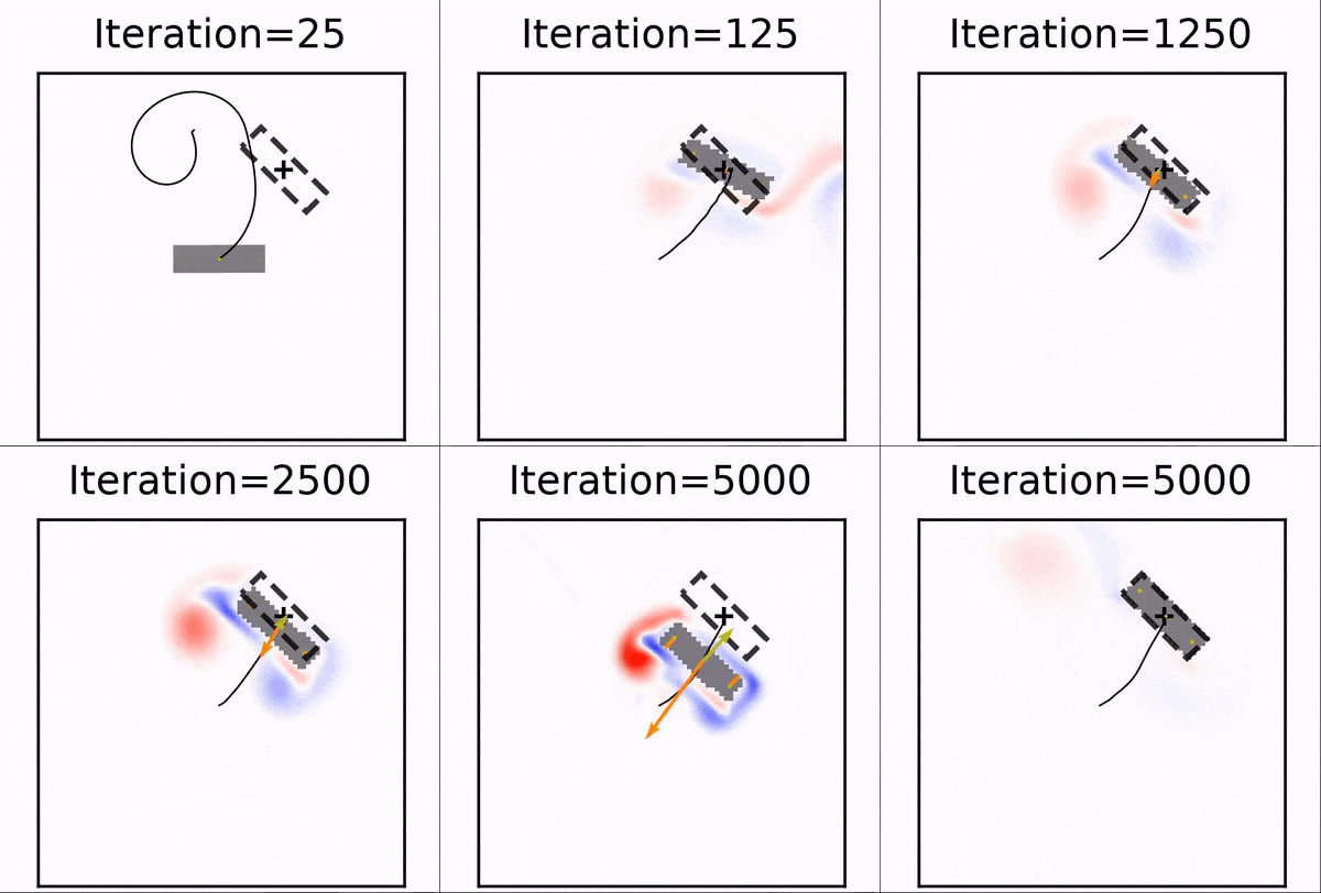
This is the source code for our paper on learning two-way control with differentiable solvers. The code is a modified version of Φ_Flow designed to investigate how differentiable solvers can be used to train neural networks to act as controllers in an unsupervised way for a fluid system with two-way coupling.

Installation

It is recommended to use a virtual environment such as conda in order to properly install the required packages.

conda create --name phiflow python=3.7
conda activate phiflow

The specific implementations for two-way coupling use the PyTorch framework, which can be installed with

conda install pytorch torchvision torchaudio cudatoolkit=10.2 -c pytorch

Navigate to the folder you would like to use to store the code and clone this repository.

git clone https://github.com/brenerrr/PhiFlow.git ./
git checkout two_way_coupling

Lastly, install all packages.

pip install . ./

Next verify that Φ_Flow is correctly installed and can access PyTorch.

python tests/verify.py

Inputs required to run most scripts are grouped in the file neural_control/inputs.json.

Generate Initial Conditions

Simulations used as initial conditions are created by executing

python neural_control/misc/generate_ic.py

Inputs necessary for generating initial conditions for training and test environments can be found in the "simulation" section of neural_control/inputs.json. All initial conditions used in our paper can be found on storage/ics/.

Training

Training neural networks as controllers using the differentiable simulator is done by executing

python neural_control/neural_networks/train_unsupervised.py path/to/export/folder/

The network is trained by minimizing the following loss function

$$L = O + V + E$$

$$O = \frac{\beta_{xy}}{l}\sum_{n=0}^{l-1}|e_{xy}^n|^2 + \frac{\beta_{\alpha}}{l}\sum_{n=0}^{l-1} |e_{\alpha}^n|^2$$

$$V = \frac{\beta_{\dot{x}}}{l}\sum_{n=0}^{l-1}\frac{|\dot{x}^n|^2}{\beta_{prox}|e_{xy}^n|^2 + 1} + \frac{\beta_{\dot{\alpha}}}{l}\sum_{n=0}^{l-1}\frac{|\dot{\alpha}^n|^2}{\beta_{prox}|e_{\alpha}^n|^2 + 1}$$

$$ E = \frac{\beta_F}{l}\sum_{n=0}^{l-1} |F_c^n|^2 + \frac{\beta_T}{l}\sum_{n=0}^{l-1} |T_c^n|^2 + \frac{\beta_{\Delta F}}{l}\sum_{n=0}^{l-1} |F_c^n-F_c^{n-1}|^2 + \frac{\beta_{\Delta T}}{l}\sum_{n=0}^{l-1} |T_c^n-T_c^{n-1}|^2 $$

where $\dot{x}$ and $\dot{\alpha}$ represent velocities, $e$ errors, and $F_c$ and $T_c$ control efforts. $\beta$ are hyperparameters that weigh the contribution of each term.

Intermediate models are saved during training before all iterations are performed as trained_model_####.pt, where #### is a model index.

All parameters for training are set in inputs.json, especially in the "unsupervised" session.

A schematic of the differentiable solver training: Blue arrows represent the forward pass while red ones illustrate the flow of gradients. Importantly, the loss signal is backpropagated through l simulation steps to provide policy P with long-term feedback about the flow environment.

Tests

Before running the tests, it is necessary to generate the tests.json that contains all tests parameters by running

python neural_control/testing/generate_tests.py

After that, test simulations can be performed by executing

python neural_control/testing/test_networks.py path/to/model/folder/ model_index tests_id

The table below summerizes all tests available with their respective IDs.

Tag	Test ID	DoF	Re	N Simulations	Inflow	Buoyancy	Forcing
BaseNR	1	2	1000	20
BuoyNR	2	2	1000	5		✔
Base	3	3	1000	20
Inflow	4	3	3000	5	✔
InBuoy	5	3	3000	5	✔	✔
Hold	6	3	3000	5	✔	✔	✔

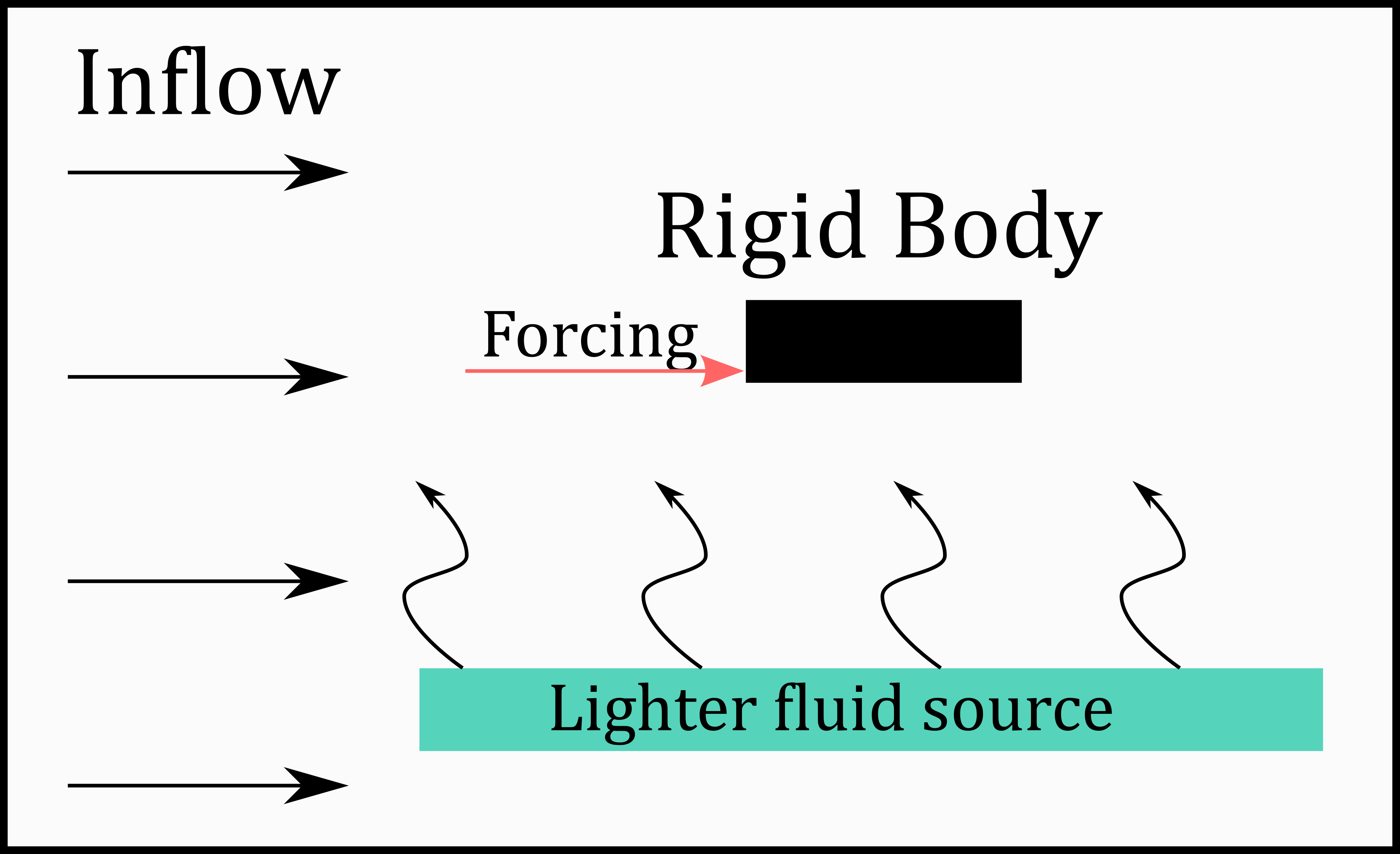
Schematic of tests environments.

After running the desired tests, calculate the metrics with

python neural_control/misc/group_frames.py /path/to/model/folder/
python neural_control/misc/calculate_metrics.py /path/to/model/folder/

This will calculate all metrics and export them to /path/to/model/folder/tests/test#_#/metrics.json.

A google colab notebook showing the overall workflow can be accessed here.

Visualization

Simulations can be quickly visualized with an interactive data visualizer GUI with

python neural_control/visualization/data_visualizer.py

When loading the GUI for the first time, after inserting the path to the directory containing the models folders, click on "Update paths" in order to update the models folder options menu.

The folder structure of the example above is set the following way

storage
│
└───diff_2dof
    │   inputs.json
    |   trained_model_0010.pt
    |
    └───tests
    |   │
    |   └───test2_10
    |       │   metrics.json
    |       |
    |       └───data
    |
    └───data (training data)

If "Test Data" is not ticked, the GUI will try to plot the "data" folder directly at the model folder (training data) instead of the one of the chosen test.

Fields

Contour plots can be generated for a specific snapshot from a test with

python neural_control/visualization/plot_fields.py path/to/storage/ test_id snapshot --folders model_folder

For example, the command below generates the vorticity contour of all simulations from test 5 at timestep 3900 located in the folder diff_3dof.

python neural_control/visualization/plot_fields.py path/to/storage/ 5 3900 --folders diff_3dof

All figures are saved on path/to/storage/figs.

Supervised Learning

A dataset must be first created in order to train a controller in a supervised way by running

python neural_control/neural_networks/generate_dataset.py

Make sure that initial_conditions_path from the supervised section of inputs.json has the correct path to the initial conditions folder. Also, the dataset will be stored in the folder dataset_path from the supervised section.

After the dataset is generated, a model can be trained with

python neural_control/neural_networks/train_supervised.py path/to/storage/folder/

The training losses are logged in path/to/storage/folder/ folder and can be visualized with TensorBoard.

Reinforcement Learning

Networks trained via reinforcement learning algorithms were also considered in this work. The code used for that is derived from this branch and can be found here. It utilizes the stable-baselines3 framework for training and the two-way-coupling simulations as the environment.

A fully trained model can be found in storage/trained_models/rl_2dof/.

Publications

• Control of Two-way Coupled Fluid Systems with Differentiable Solvers, Brener Ramos, Felix Trost, Nils Thuerey, arXiv 2022.