-
Notifications
You must be signed in to change notification settings - Fork 73
Flocking
Scripts to compute transfer entropy between interacting pairs in flocks
Demos > Flocking/Swarming scripts
This demo, distributed at demos/octave/FlockingAnalysis, provides a set of scripts to compute (pairwise) transfer entropy between pairs of individuals in a swarm or flock. The analysis takes samples from pairs of individuals who are within a given radius of eachother at specific time steps (assuming that interactions only occur within such a radius). We assume that all individuals in the flock/swarm are homogeneous agents, and therefore bring all of the sample interactions into a single calculation, providing an average transfer entropy for a representative pair interaction. The scripts also compute local transfer entropies for every observed within-radius interaction within the data. Active information storage is also computed.
This method of computing transfer entropy for a flock/swarm is detailed in the following papers:
- X.R. Wang et al., "Measuring Information Storage and Transfer in Swarms", in Proc. Eleventh European Conference on the Synthesis and Simulation of Living Systems (ECAL 2011), Paris, 2011. Published in Advances in Artificial Life, ECAL 2011, by Massachusetts Institute of Technology, ISBN 978-0-262-29714-1, 2011, pp. 838-845 -- then
- X.R. Wang et al., "Quantifying and Tracing Information Cascades in Swarms", PLoS ONE, vol. 7, no. 7, e40084, 2012; doi: 10.1371/journal.pone.0040084 -- then
- E. Crosato et al., "Informative and misinformative interactions in a school of fish", Swarm Intelligence, vol. 12, no. 4, pp.283-305, 2018; doi:10.1007/s11721-018-0157-x (or preprint arXiv:1705.01213) -- which is the final definitive version
We have used this method, and in particular these scripts, to analyse tracking data from fish in the following papers (and more):
- A. Ward et al., "Cohesion, order and information flow in the collective motion of mixed-species shoals", Royal Society Open Science, vol. 5, no. 12, 181473, 2018; doi:10.1098/rsos.181132.
- M. Kent et al., "Speed-mediated properties of schooling", Royal Society Open Science, vol. 6, no. 2, 181482, 2019. doi:10.1098/rsos.181482
- M.J. Hansen et al., "The effect of predation risk on group positioning behaviour and information flow during repeated collective decisions", Animal Behaviour, in press, 2021; doi:10.1016/j.anbehav.2021.01.005 -- contains some more technical details than the others in this list.
- A.L. Burns et al., "Self-organization and information transfer in Antarctic krill swarms", Proceedings of the Royal Society B, vol. 289, p. 20212361, 2022.
I've summarised our method and some of these applications in a presentation at CCS 2019.
Swarm/flocking data has many differences to regular multivariate time series, and it doesn't make a lot of sense to treat them as a standard time series. These issues include:
- Each individual may only be tracked for a short period out of the total tracking time series. This leads to missing data if you try to compute transfer entropy between time series for any two individuals.
- You could select shorter parts of the time series when pairs of individuals are in frame, although they are usually only within interaction range for a few frames out of the whole time they are together in view. When they are far apart, it doesn't make sense to examine a potential interaction.
- You could select shorter time series when pairs are both in frame and within interaction range. But you'll be left with very little data for each pair.
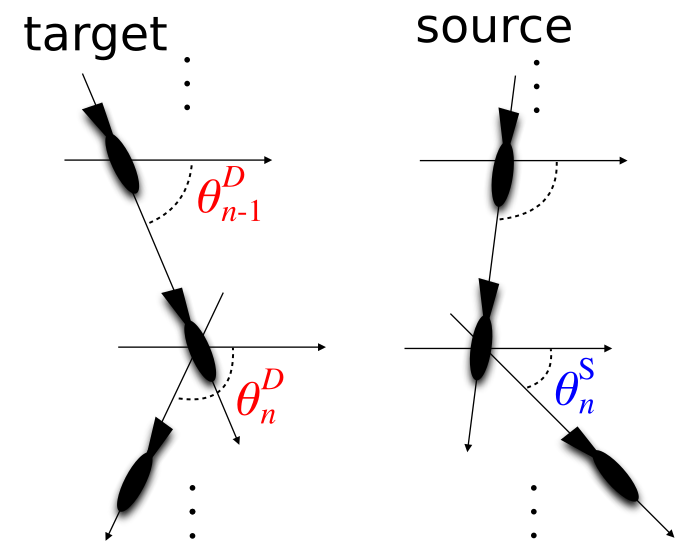
- The relevant information for an interaction between two individuals in a flock/swarm is not directly in their absolute position/velocity (which is the raw tracking data we usually have). Instead, the relevant information sits in other derived variables -- i.e. relative headings, relative distances, etc. Think of how one individual in the swarm updates it's heading/speed in a 3-zone model -- it uses relative headings and velocities of its near neighbours, not their absolute headings / velocities.

In order to address these issues, our approach as detailed in the papers above:
- Extracts sample observations of source-target interactions from all observed pairs with a given range in the tracking view at each timestep, extracting the relative headings / velocities and heading updates (as detailed above). This pulls the relevant variables for examining how relative information from the source adds predictive information about the target individual's state update.
- Uses all of those sample observations -- across all sampled source-target interactions -- to make a single information-theoretic calculation of transfer entropy. This assumes that all individuals are behaving in a homogeneous fashion when presented with a relative source individual, allowing us to hone in on the relevant information and combine across all pairs to increase statistical power (i.e. avoid the issue of having too few time samples for any pair).
This approach is used to return an average transfer entropy across all sample source-target interactions in the data set, and also a local transfer entropy for each of these samples.
We provide loaders for tracking data in some flat file formats, but we also faciliate you writing your own loaders for your own file formats to then provide the data in a compatible format. See details in "Step 3 -- set up your properties file" below.
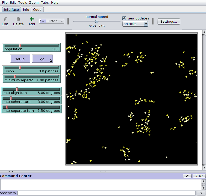
For the purposes of a demonstration, we will generate sample data using the NetLogo model distributed in the partner jidt-cc-extras repo at demos/octave/FlockingAnalysis/NetLogoExample/Flocking.nlogo (download from the file in jidt-cc-extras repo). This NetLogo model, which simulates simple 3-zone flocking behaviour in 2D, has been adapted from the original CC BY NC SA 3.0 licensed Flocking model distributed with NetLogo, and is released under the same license.

The fastest way to generate sample flocking data via this NetLogo model is as follows:
- Open this script using NetLogo v6 (some tweaks to the file I/O may be required for NetLogo v5)
- Click the go continuous button.
- Stop the simulation after a few hundered or a thousand time steps.
The model will have written files positionsx.txt, positionsy.txt and headings.txt in thesame folder, which each record the eponymous data for every member of the flock: each row is one time step, each column is for one individual in the flock - read the NetLogo code to see more details on the format. It will stop appending to these files after 4000 time steps, so you can stop the simulation after that - that will be an awful lot of data anyway, you don't need it to run that long.
The data will be of better quality if we have multiple shorter runs from different initial conditions. To do that, you can:
- Stop the simulation after say 300 time steps, then rename those files to e.g.
positions1x.txt,positions1y.txtandheadings1.txt. - Then click the Setup button to reinitialise the simulation and
- Click go again to generate new data files -- Stop the simulation after another say 300 time steps (doesn't have to be exactly the same number).
- Keep looping on stopping the simulation and renaming the files until you have say 5 repeat runs of approximately 300 time steps each.
This is a significant amount of data, which is good for nice results ... but to check if you have it working, try first to run the analysis below with just one file set with say 50 time steps.
Your transfer entropy analysis requires three separate resources, which can be in three separate folders:
- The analysis scripts at
demos/octave/FlockingAnalysisin the JIDT tree; - A properties file describing the parameters for this analysis. If you are running with the NetLogo flocking example above, the sample properties file is distributed at
demos/octave/FlockingAnalysis/NetLogoExample/loadProperties.m(see in repo). - Your data (as per the above step). It can be in the same location as the properties file, or else the location folder can be set in that script.
Your loadProperties.m file contains all of the parameter settings your analysis needs - aside from setting these properties, you shouldn't need to tweak any of the code for a standard analysis.
Have a look through the loadProperties.m file to see what parameters you can change -- all of those are documented in that sample properties file in some way. They include:
- location of the data file(s) (
properties.files), - which matlab function file to use to read these data files into our standard format or you can add your own file reader (
properties.loadScript). The comments for this sample properties file also describe how to handle individuals not being present at each time step in the data; - where to write the results (
properties.resultsFile), - distance within which to consider a pair as interacting (
properties.pairRange), - whether to make the transfer entropy calculation based on heading or speed or both (
properties.headingcalcandproperties.speedcalc) and whether to include relative source position (properties.includeSourcePositionInTransfer), - which transfer entropy estimator to use from Gaussian or KSG (
properties.estimator), and - which transfer entropy parameters to set (e.g. target history dimension k in
properties.k) or else a range within which to optimise these parameters (e.g.properties.kRange), etc. - whether to include serial or dynamic correlation exclusion (aka Theiler window for nearest neighbour methods) in the information theoretic estimation (set
properties.jidt.autoDynamicCorrelationExclusion = true;). Note that this setting will require the Econometric Toolbox to be installed in Matlab.
Your next step in an analysis is to check that the properties are all ok in the loadProperties.m file for this experiment.
Probably the most important property to check when you change to running your own analysis later on will be how the data files are named, located and accessed. The naming convention for your files may also depend on which script you specify to load your data into our standard format. The file is currently set up for our NetLogo example, which uses loadseparatexy.m to read in the data files; this script take a template as the file name ('positions%s.txt') and then substitutes 'x' and 'y' for the '%s' placeholder to make the two filenames it required. There are other file loaders available for other input file formats (see the load*.m files), or you can write your own loader and specify it via the loadScript property. See the existing file loaders for the data format we require these loaders to return.
You will also see in the properties file that if you have several data files here instead of just one, this can be handled by specifying a cell array or list in the files property. For the NetLogo example above, if you generate multiple data files as per the suggestion, you would to change the value of files line to be, e.g.:
properties.files = {'positions1%s.txt', 'positions2%s.txt', 'positions3%s.txt', 'positions4%s.txt', 'positions5%s.txt'};You can run a sample analysis as follows:
- In Matlab or Octave, change to the folder where your
loadProperties.mfile for the current experiment resides (for the above NetLogo example this isdemos/octave/FlockingAnalysis/NetLogoExample/). You will run all of the following analysis scripts from this location. - At the Matlab prompt, manually add the location of the analysis scripts (which are at
demos/octave/FlockingAnalysisin your JIDT distribution) usingaddPath. For the NetLogo example, the scripts should still be in the folder above and so you would run:addpath('..'); - Load in the properties for this experiment by running the
loadProperties.mfile. You will need to rerun this whenever you change any parameters so that they take effect.loadProperties - Calculate the information theoretic quantities (transfer entropy and active information storage) and save them to the results file named in
loadProperties.m:This will finish by printing out an average transfer entropy across all interacting pairs, and storing all of the relevant results (including relative headings and positions, optimised parameters, average transfer entropy, and local transfer entropies for each observation of an in-range interaction) in the specified results file.runAnalysis(properties) - Read the results from the results file and plot the local TEs against relative source-target position:
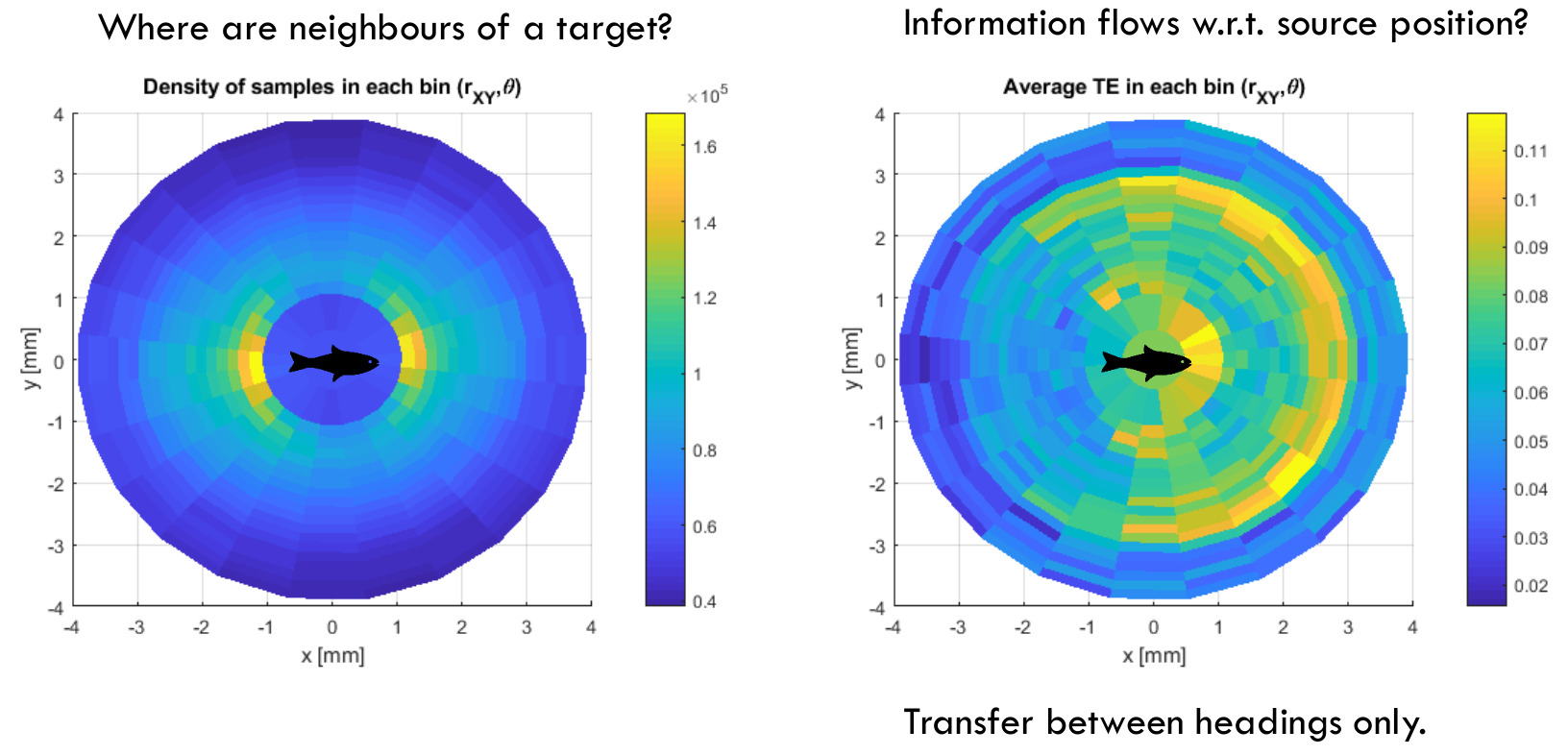
That plotting file makes a visualisation of the average transfer entropy with respect to relative position of the source to a target. That's a different type of visualisation to those in our paper Crosato et al. above. You should be able to follow how this plot file is reading the local transfer entropies from the results file though if you want to make any other type of visualisation, such as videos of local TE such as we make in Wang et al above.
plotLocalTEs()
- Another way of post-processing the data is to read the results from the results file and plot the local TEs (averaged for each target) against target position at each time step:
watchLocalTEs()
A sample visualisation of the average transfer entropies found with respect to relative source position to the target is generated from the NetLogo 3-zone flocking model as follows:

We can make several interesting observations from the following:
- The transfer entropy is observed to be at elevated levels within an interaction radius of 3 units, and drops quickly to the background noise level outside of this. This can be explained in that the outermost interaction radius in the NetLogo model was set to 3, however we included interacting pairs within a radius of 4 in this example analysis. Clearly there is insignificant information flow between pairs examined who are separated by more than the causal radius.
- There are two "hot zones" for information transfer here, a semi-ring in front and to the side of the target individual around a radius of 1, and another semi-ring in front and to the side of the target individual just under a radius of 3.
- The hot zone around a radius of 1 appears to be capturing information flows associated with the triggering the "separate" action of the target individual (minimum radius of 1 is set)
- The hot zone just under a radius of 3 appears to be capturing information flows associated with new neighbours entering the interaction radius of 3 units. In contrast to closer neighbours who have likely been influencing the target already over a number of time steps, these outer neighbours may not have been influencing the target at the previous time step and so their new influence has a novel effect on the target's state update, manifesting as stronger information flows.
- Note that these hot zones are specifically in front and to the side of the target fish, but not so much behind it. Yet the align-cohere-separate 3-zone flocking rules apply to neighbours wherever they are within radius. As such, the smaller information flows from behind the fish are an emergent effect here, and are not due to any reduced vision behind the fish. This is likely because neighbours entering the separate zone or outer interaction radius, and causing the large information flows described above, are overwhelmingly likely to enter form the front or side of the target: since the target is moving forwards, and all fish have constant velocity in this example, it is difficult to arrange such a zonal entry from behind the target.
JIDT -- Java Information Dynamics Toolkit -- Joseph Lizier et al.
- Home
- Getting started
- ImplementedMeasures
- Demos
- Course (long)
- Tutorial (short)
- Non-Java environments
- FAQs
- Miscellaneous
- For serious developers!
- Publications resulting