-
Notifications
You must be signed in to change notification settings - Fork 44
First steps
The recommended way to install Helios++ is via the conda package manager.
The following software is required for installation of Helios++:
- a Conda installation, we recommend mamba, micromamba, or miniconda.
Helios++ can then be installed with:
conda install -c conda-forge helios
If you intend to contribute to the development of HELIOS++, we recommend a locally compiled version using these instructions.
git clone https://github.com/3dgeo-heidelberg/helios.git
cd helios
conda env create -f environment-dev.yml
conda activate helios-dev

# On Linux, the following line is recommended, to go with a Conda-provided compiler.
# We had issues with incompatible system compilers before.
conda install -c conda-forge gcc gxx

python -m pip install --no-deps -v -e .
If you explicitly require a manual CMake build, you can create it like this:
mkdir build
cd build
cmake -DCMAKE_PREFIX_PATH=<conda-env-root> ..
make
To avoid unexpected behavior, we suggest to run the test cases after installation. To do this, open a terminal and clone the repository. Then navigate to the HELIOS++ root directory and run run\helios --test:
git clone https://github.com/3dgeo-heidelberg/helios.git
cd helios
run\helios --test
> run\helios.exe --test
TEST Randomness generation test                           [PASSED]
TEST Noise sources test                                   [PASSED]
TEST Discrete time test                                   [PASSED]
TEST Voxel parsing test                                   [PASSED]
TEST Ray intersection test                                [PASSED]
TEST Grove test                                           [PASSED]
TEST Serialization test                                   [PASSED]
TEST Asset loading test                                   [PASSED]
TEST Survey copy test                                     [PASSED]
TEST Plane fitter test                                    [PASSED]
TEST LadLut test                                          [PASSED]
TEST Platform physics test                                [PASSED]
TEST Functional platform test                             [PASSED]
TEST Scene part split test                                [PASSED]
TEST Expression tree test                                 [PASSED]
TEST Rigid motion test                                    [PASSED]
TEST Fluxionum test                                       [PASSED]
TEST Energy models test                                   [PASSED]
TEST HPC test                                             [PASSED]
Be sure to also check if the return code is zero (environment variable ERRORLEVEL), e.g. on Windows:
> echo %ERRORLEVEL%
0
In the HELIOS++ repo, you will also find a data subfolder with a number of example surveys, scanners, platforms and scenes. They provide a good starting point for experimentation and are required to pass some of the test cases.
Starting HELIOS++ is done in a command line by telling it where to find the survey file.
Type
helios [survey-file]
and hit the Enter button to start the simulation.
The software has a modular architecture, where the simulation assets (i.e. platform, scene and scanner) are read from XML files and linked scenepart files. [survey-file] is the absolute or relative path to a survey XML file. In this XML file, paths pointing to the scene XML, the platform XML and the scanner XML are provided. If those paths are relative (recommended for sharing), their base directory needs to be in the list of HELIOS++ assetsPaths. This way, it can be sufficient to only specify filepaths in the XML survey and scene files and then adding seach folders to the assetPath list. To do so, add one or multiple file paths via the --assets argument, e.g.,
helios [survey-file] --assets <path/to/my/scenes> --assets <path/to/my/sceneparts>
Sample scenes, platforms and scanners are provided in the data directory. For example, from the HELIOS++ root directory, run
helios data\surveys\demo\tls_arbaro_demo.xml
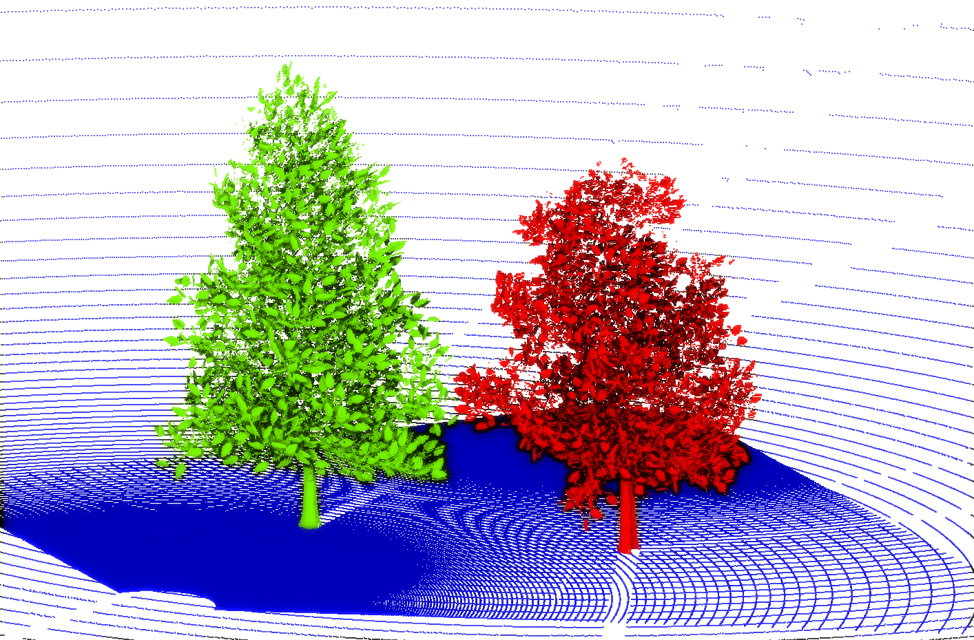
which will run a simulation of a TLS scan of two trees from two scan positions. The output will be created in the output/Survey Playback/Arbaro Demo - folder under the timestamp of the simulation start. This point cloud can be visualized e.g. using Cloud Compare, and may look like this:

To print the HELIOS++ help message, type:
run\helios -h
This gives you an overview of additional, optional arguments.
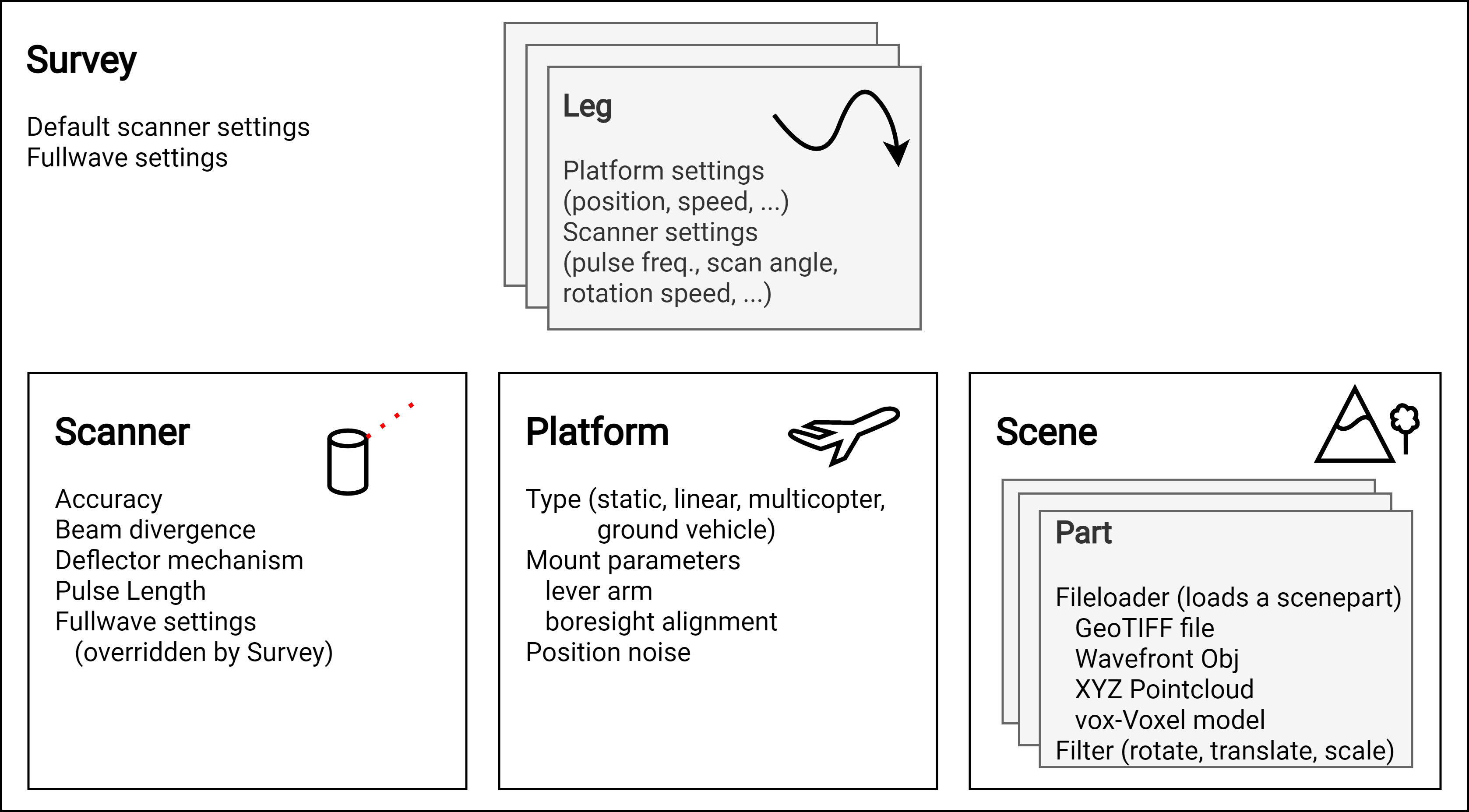
The following figure provides a general overview of the main HELIOS++ XML files, their content, and their connection:

In the survey XML, scan positions or way points are configured and full waveform settings, platform settings, and scanner settings can be controlled.
The scene XML links to the different geometry parts, which can be of different types such as polygon meshes, georeferenced rasters (GeoTiff), point clouds or voxels. Different parameters and filters can be passed to define how to load and pre-process the linked files, including transformations such as translation, rotation and scaling of individual scene parts. More details are listed in on the Scene subpage.
The platform XML contains the definition of different platforms, such as a stationary tripod for terrestrial laser scanning simulations, vehicles for mobile laser scanning simulations and aircrafts for airborne laser scanning simulations. A number of platforms are predefined (tripod, quadcopter, Cirrus SR-22, ...) and can be extended. See the platforms.xml file in the data folder.
The scanner XML contains scanner specifications like beam divergence, accuracy, deflector type, pulse frequency or pulse length. Similar to the platforms, a number of scanners are predefined in scanners_als.xml and scanners_tls.xml in the data-folder.
HELIOS++ comes with a folder structure which helps in storing and finding these compartments. It is therefore recommended to work in the provided folder structure:

The paths pointing from the survey XML file to the other XML files can be set relative or absolute. Note that for relative paths, HELIOS++ will search in any paths that are in the assetPath list, which is also logged when you run a survey. By providing the base directories using the --assets argument, your files can also be located in different locations.
The software loads the geometries and performs a simulation according to the specified input configurations. By default, the output is written to output/Survey Playback (see Optional Argument --output). Separate folders are created for each survey and for each time the survey is executed. Points are written to XYZ ASCII files (default) or LAS files (using the --lasOutput argument), with one file per leg (i.e. per scan position, flight line or path), respectively. Optionally, the full waveform can be exported, by adding --writeWaveform as command line argument.
Accordingly, a more elaborate example to start a simulation would be:
run\helios data\surveys\demo\tls_arbaro_demo.xml --lasOutput --writeWaveform --seed 42 -j 1
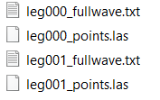
which creates a reproducible simulation (because of fixed seed, cf. Controlling Randomness) , writes LAS output files and additionally writes the fullwave signal into ASCII files. The result folder will look like this:

If you want to export the trajectory, you can provide the trajectoryTimeInterval_s="0.01" attribute in the <scannerSettings [...]> tag in the survey XML. The position and attitude of the platform will then be written to an ASCII output file for each leg every 0.01 seconds (depending on the value of the attribute). For static platforms (TLS), this attribute is ignored. See the separate page Output for details on the file formats.
We have created a number of example jupyter notebooks that show you how to use HELIOS++ and especially its XML syntax and Python bindings:
 |
Two highly detailed tree models (loaded from .OBJ files) are scanned from two positions with a terrestrial laser scanner (TLS). |
 |
A wheat field (loaded from .OBJ files) is scanned from a tractor with mobile laser scanning (MLS). |
 |
A scene with different simple geometries (toyblocks, loaded from .OBJ files) is scanned by means of mobile laser scanning. |
 |
UAV-based laser scanning (ULS) is conducted over a toyblock scene. This example shows how to define the survey and the scene in a single XML file. |
 |
With airborne laser scanning (ALS), the terrain of Heidelberg (Germany) is scanned. For the virtual 3D scene, a digital terrain model (DTM) is loaded from a GeoTIFF. |
 |
Again, Heidelberg is scanned using a DTM of Heidelberg. This time, the airplaine holds a constant height above the ground by creating many support points with different heights. The many small segments are grouped to three strips using the stripId parameter. |
 |
A point cloud (XYZ ASCII file) is loaded to a voxel model with HELIOS++ and then scanned by TLS. Voxel normals are computed from the point cloud, which affect the beam incidence angles and hence the computed intensities. |
 |
Different modes for 3D (vegetation) modelling with detailedVoxels are demonstrated for a single tree. Both ULS and ALS simulations are conducted. |
 |
TLS is conducted using a Livox Mid-70 with a risley prism, resulting in a non-repeating, retina-like scanning pattern. |
 |
A toyblocks scene is scanned by ULS scanning using a Livox Mid-70 sensor. |
 |
A toyblocks scene is scanned by ALS using the Livox Mid-100, a device composed of three Mid-40 units. |
 |
The configuration of multi-channel scanners is demonstrated with the Velodyne Puck, which has 16 channels. A "box scene" is used for visualisation and debugging purposes. |
 |
ALS is simulated using a trajectory as input, from which platform position and platform attitude at a given time is read. HELIOS++ interpolated between the time values. The trajectory interpolation is demonstrated with simple examples using the box scene. |
 |
An urban scene with two moving vehicles is scanned using mobile laser scanning (MLS) from a car. The scene is dynamic, which means that the scene parts undergo rigid motion (translation, rotation) during the scan simulation. |
 |
A tree with fluttering leaves is scanned using terrestrial laser scanning (TLS) from multiple scan positions. Leaf flutter is implemented by rotating the leaves during the virtual scans, see Dynamic Scenes. |
 |
An ALS simulation over a toyblocks scene is repeated for four epochs ("swaps"). Each scene part undergoes changes between the "swaps", where either the geometry is replaced, the coordinate transformation is modified, or the scene parts disappears, see Scene Swaps. |


