The relatively recent mainstream availability of complex algorithms and computationally efficient hardware is creating a platform for new innovations never before available to the scientific computing world. Since the development of computer systems, computing times have been drastically reduced, making more complex computations feasible. The continuous cycle of improvements in computation speeds and hardware leading to ever more complex computations can be seen in the scaling of hardware to meet these more complex computation goals. A resolution to this cycle can be found in the utilization of GPU's in high-performance computing for Machine learning and deep learning algorithms. Most of the complex computing strategies can be simplified into basic linear algebra operations such as addition, multiplication, subtraction, inversion and such. Out of the listed operations, matrix multiplication and inversion are the most computationally expensive operations.
Most matrix operations are performed sequentially on the CPU resulting in computation time that scales with the size of the matrix as a factor θ(n3). Hence, computation cycles and duration of time to be allocated towards computation is proportional to the size of matrices under the constrained hardware with limited cache memory and RAM. The same problem still exists with multicore systems or distributed systems due to the threshold on the resources mentioned. On the other hand, a GPU is composed of several thousand cores, combining to provide the user with several GBs of computational memory compared to the MBs provided by CPU cache memory. The distributed computing this configuration provides enables parallelism across GPU cores and allows a super fast flow of data resulting from incredibly high bandwidth. This distribution across multiple cores amounts to massively reduced computation time as the device is able to scale its performance with data size.
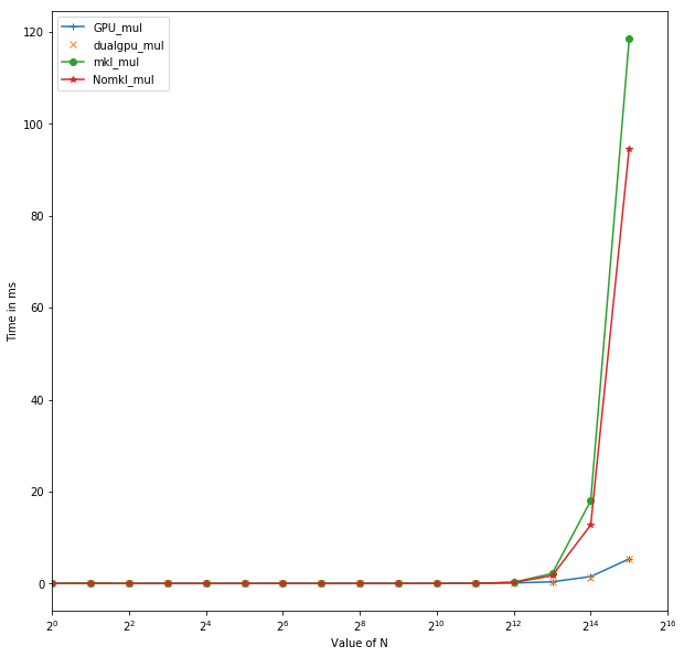
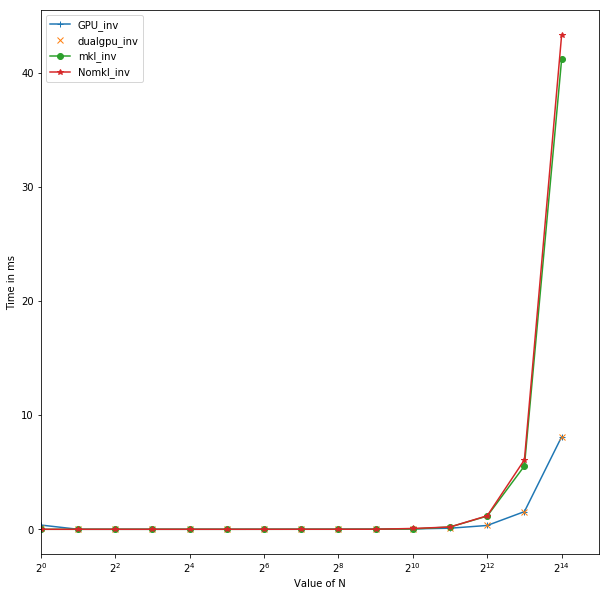
The enormous gains in computation time should give researchers a valid reason to switch from CPUs to GPUs for computationally heavy operations where the CPU-based operations do not scale with the data at a constant rate. Utilization of this methodology will provide enormous benefits for the computationally heavy domains such as machine learning, deep learning, linear algebra, optimization, data structures, etc. To illustrate this statement, we've included some benchmarks run on the Xena system at CARC using intensive linear algebra operations, i.e., matrix multiplication and matrix-inversion, on a CPU only compared to CPU utilizing the GPU as well.
The CPU version was deployed on a multicore processor with 16 cores and 64GB of RAM with using numpy arrays in python. The GPU Version was deployed on NVIDIA Tesla K40 with 11GB of GPU memory using Tensorflow. Here the CPU implementations were carried with two different types of numpy compilations. mkl_mul stands for multiplication operation carried with numpy compiled with math kernel library. Nomkl_mul stands for the numpy without math kernel library. mkl based numpy was installed in an anaconda enviroment using conda to install numpy whereas the numpy installed with pip doesn't integrate math kernel library. Xena has nodes with single GPU and dual GPU. Dual GPU node offers users 2x11GB of computational GPU memory which allows the use of a larger batch size and double the number of cores for faster implementation of highly complex models with a large number of parameters. The GPU_mul corresponds to multiplication operations utilizing single GPU node and dualgpu_mul corresonds to the one utilizing a dual GPU node. Another interesting benchmark was performed for inversion operations similar to those done for multiplication
Fig 1. Time for Matrix Inversion vs size of Matrix N
Fig 2. Time for Matrix Multiplication vs size of Matrix N
The implementations can be found here.
Tensorflow is an open source deep learning library provided by Google. It provides primitives for functions definitions on tensor and a mechanism to compute their derivatives automatically. It uses a tensor to represent any multidimensional array of numbers.
Comparision between Numpy and Tensorflow
TensorFlow's computational housing is a tensor, similar to Numpy's housing of data in Ndarray's making both of them N-d array libraries.
However, Numpy does not offer a method to create tensor functions and automatically compute derivatives, nor does it support GPU implementation. Thus, for processing data of higher dimensions,Tensorflow outperforms Numpy arrays due largely to its GPU implementations.
Numpy vs Tensorflow Implementations
Numpy Implementation of Matrix Addition
	import numpy as np
	a=np.zeros((2,2))
	b=np.zeros((2,2))
	np.sum(b,axis=0)
	a.shape
	np.reshape(b,(1,3))
Tensorflow Implementation of Matrix Addition
	import tensorflow as tf
	tf.InteractiveSession()
	a=tf.zeros((2,2))
	b=tf.ones((2,2))
	tf.reduce_sum(b,reduction_indices=1).eval()
	a.get_shape()
	tf.reshape(b,(1,3)).eval()
It is important to note that tensorflow requires explicit evaluation, i.e, tensorflow computation defines a computational graph which only gets initialized with values after a session has been evaluated.
Numpy for example
a=np.zeros((2,2)) ; print(a)
will immediately give the value of "a".
However, for tensorflow:
	a=tf.zeros((2,2))
	print(a)
will not return the value of "a" until it is evaluated with
print(ta.eval())
So It is important to understand how tensorflow works and initializes the environment.
Tensorflow uses a "session object" which encapsulates the environment in which the tensors are evaluated.
A Tensorflow (tf) session for performing multiplication is demonstrated below:
	a= tf.constant(9999999)
	b=tf.constant(111111111)
	c=a*b
	with tf.Session() as sess:
	     print(sess.run(c))
	     print(c.eval())
Tensorflow firstly structures the program, creates a graph integrating the variables, and uses session to exectute the process.
*** Tensorflow Variables *** Similar to other programming language variables, tensorflow uses a variable object to store and update the parameters. They are stored in memory buffers that contain tensors. TensorFlow variables must be initialized before they have values! This is in contrast with constant tensors:
	W=tf.Variable(tf.zeros((2,2)), name="weights")
	R=tf.Variable(tf.random_normal((2,2)), name="Random_weights")

	with tf.Session() as sess:
	        sess.run(tf.initialize_all_variables())
		print(sess.run(W))
		print(sess.run(R))
Converting numpy data to tensor:
	a=np.zeros((3,3))
	t_a=tf.convert_to_tensor(a)
	with tf.Session() as sess:
		print(sess.run(t_a))
For scalable variables for performing operations we can use tf.placeholder which defines a placeholder and provides entry points for the data to be viewed in a computational graph. feed_dict is used in the below example to map from tf.placeholder variables to data (np arrays, list, etc).
	input1= tf.placeholder(tf.float32)
	input2 = tf.placeholder(tf.float32)
	output = tf.multiply(input1, input2)
	with tf.Session() as sess:
		print(sess.run([output], feed_dict={input1:[7.], input2:[2.]}))

