End-to-end content based fashion product recommendation engine based on visual similarity of items.
This blog is inspired by the research paper published by Myntra

Have you ever looked at a model and wondered if you could ever look like him/her? Ever wondered how to develop a good fashion sense? Don't worry this blog has a very elaborate (a bit much if you ask me) solution to both of those questions. The rise of e-commerce websites in India has led to an increase in online shopping throughout the country. Fashion items are the most sought after in the e-commerce market. A robust, effective, and efficient recommendation system for fashion items could lead to an increase in revenue, better customer engagement, and experience. What makes this approach novel is the ability to detect multiple products from a given Product Display page and recommend similar items to the user. A Product Display Page (PDP), is a web-page that presents an image of the product/products worn by a model or a standalone picture of the product in a plain background. This approach helps the user to not only look for the relevant item in a single category but also to match those items with other items that go well with the specified product. In simple words, thanks to the advancements in computer vision, you can copy the look of your favourite celebrity by just using an image of that look.
The proposed solution is a Content-Based recommendation system that involves various modules that carry specific tasks that help in achieving the overall goal. For the system proposed in the published article by Myntra the first module consists of the Human Key Point Detection, looks for specific human key points like the ankle and the eyes in order to classify the image as a full-shot image i.e. an image that consists of the full body of a model, however the solution proposed in this blog skips this step, instead we'll recommend items using all the fashion products detected in an image. For better product recommendation we'll first try to determine the gender of the person in the query image. The pose can either be front, back, left, right or detailed. After determining the gender, the input is fed is then fed to the next module, it’s an Object Detection module trained to identify objects from these broad categories - top-wear, bottom-wear, and foot-wear. The goal of this module is not just the identification of these objects in the image but also to localize the objects with bounding-boxes. Once the bounding boxes are obtained for a certain object, that part of the image is cropped and the semantic embeddings for the cropped image are obtained, which will help in identifying similar products from the catalog/database of products whose semantic embeddings are already known. We'll train a Siamese Network for generating the embeddings for the catalog of images. This system helps in automatically and efficiently recommending new items to a user who has selected or shown interest in a certain product display page.
To get started with the Fashion Recommendation Engine, we'll need a catalog/database consisting of fashion products to recommend. Unless you have a database of these items lying around we'll need to acquire this data using simple web scraping tools in python. Since we'll focus on recommending items accross various categories we'll need a diverse set of fashion products to populate the database. We can use Myntra's e-commerce website to query images using specific keywords and later save the product details for the results obtained. This way we can categorize products into various sections which would make it easier while recommeding items. We'll use Selenium package from python, its the most popular browser automation tool mainly used to carry out web-product testing. For that we'll require webdriver, for chrome users, you can get it from here, make sure the version that you download matches with the version of chrome on your computer. For more details on webscraping e-commerce websites using python follow this article "Webscraping e-commerce websites using python". After scraping the image and product urls, you either use it to download the images into your local system or save the image and product urlspair to a flat file and use it later.
# import necessary libraries
import time
from selenium import webdriver as wb

# Enter the path to your webdriver's .exe file here
wd = wb.Chrome('chromedriver.exe')

# List of search terms to use for querying from the e-commerce sites
search_terms = ["Mens Topwear", "Womens Topwear", "Mens Bottomwear", "Womens Bottomwear", "Mens Footwear", "Womens Footwear"]

# Define the Maximum number of products you want to scrape per search term
MAX_PRODUCTS_PER_CATEGORY = 1000
image_urls, product_urls = list(), list()
for search_term in search_terms:
    search_term = search_term.lower()
    query = f"https://www.myntra.com/{search_term.replace(' ', '-')}"
    total = 0
    wd.get(query)
    while total < MAX_PRODUCTS_PER_CATEGORY:
        time.sleep(3)
        products = wd.find_elements_by_class_name("product-base")
        for product in products:
            try:
                image = product.find_element_by_tag_name("img")
            except:
                continue
            image_urls.append(image.get_property("src"))
            product_urls.append(product.find_element_by_tag_name("a").get_property("href"))
    try:
        wd.find_element_by_class_name("pagination-next").click()
    except:
breakNow that we've gathered the catalog, lets do some exploratory analysis on it. The dataset consists of 10310 fashion products in various categories. The categories being:
The fashion products are not equally split among the two genders, there are 5992 Mens Products whereas as just 4318 Womens products. The plot below is a visual representation of the products split by genders.
Distribution across the categories of Topwear - 3770, Bottomwear - 3524 and Footwear - 3016.
There is huge disparity in the distribution among the type of clothing. Around 60% of the fashion items are of type casual whereas formal and party wear occupy just 30% and 10% respectively. The recommendations for casual would obviously be better considering the variety of items present in them. Here's a visual representation.
In order to recommend relevant items to the user we'll have to first detect the gender of the person present in the query image. Doing so will allow us to generate and query embeddings only on certain subsets of the catalog instead of the whole database. This will also help us in reducing irrelevant recommendations to the user based on their gender. For this task we'll make use of the Man/Woman classification dataset from Kaggle. This is a manually collected and cleaned dataset containing 3354 pictures (jpg) of men (1414 files) and women (1940 files) that includes full body and upper body images of men and women. This is ideal for our use case since we'll mostly have full body images of models wearing various fashion items. For classification we can use a ResNET50 backbone initialized with 'Imagenet' weights attached to a fully connected network that outputs the probability scores for the two classes. We'll freeze all the layers from the backbone since the task is coparitively easy to achieve and inorder to avoid overfitting to this dataset. Below is a code snippet for the model used for classification. We are abe to achieve accuracy of 95% on the test set which is decent for our use case.
from tensorflow.keras.models import Model
from tensorflow.keras.applications.resnet import ResNET50
from tensorflow.keras.layers import Flatten, Dense, Dropout, BatchNormalization

base_model = ResNet50(weights="imagenet", input_shape=(224,224,3), include_top=False)

for layer in base_model.layers:
    layer.trainable = False

x = Flatten()(base_model.output)
x = Dense(512, activation="relu")(x)
x = Dropout(0.3)(x)
x = BatchNormalization()(x)
x = Dense(128, activation="relu")(x)
x = Dropout(0.3)(x)
x = BatchNormalization()(x)

output = Dense(1, activation="sigmoid")(x)

gender_classifier = Model(base_model.input, output, name="Gender_Classifier")In order to recommend similar products we'll first need to detect all the products in a given image, and for generating the embeddings we'll need to crop out the product from an image. Object detection is one of the most interesting aspect of Computer Vision. Most object detection systems have some kind of trade off between inference speed and detection accuracy. In order to better understand object we'll need to understand a metric called 'mAP' or Mean Average Precision, for object detection whether a detection is considered correct or not depends on the IoU (Intersection over Union) threshold. The IoU score for a predicted bounding box and actual bounding box is defined as
For a pre-defined IoU threshold we can define if a detection was accurate or not if the IoU is greater than the thresold. Based on the detections Precision and Recall is defined as.
Where TP = True Positive, FP = False Positive & FN = False Negative
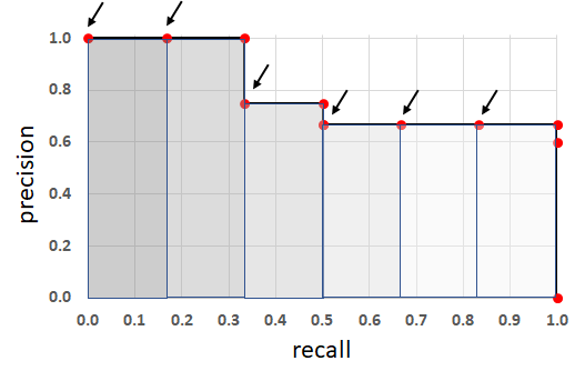
The average precision is calculated by using the Area Under the Precision and Recall Curve.
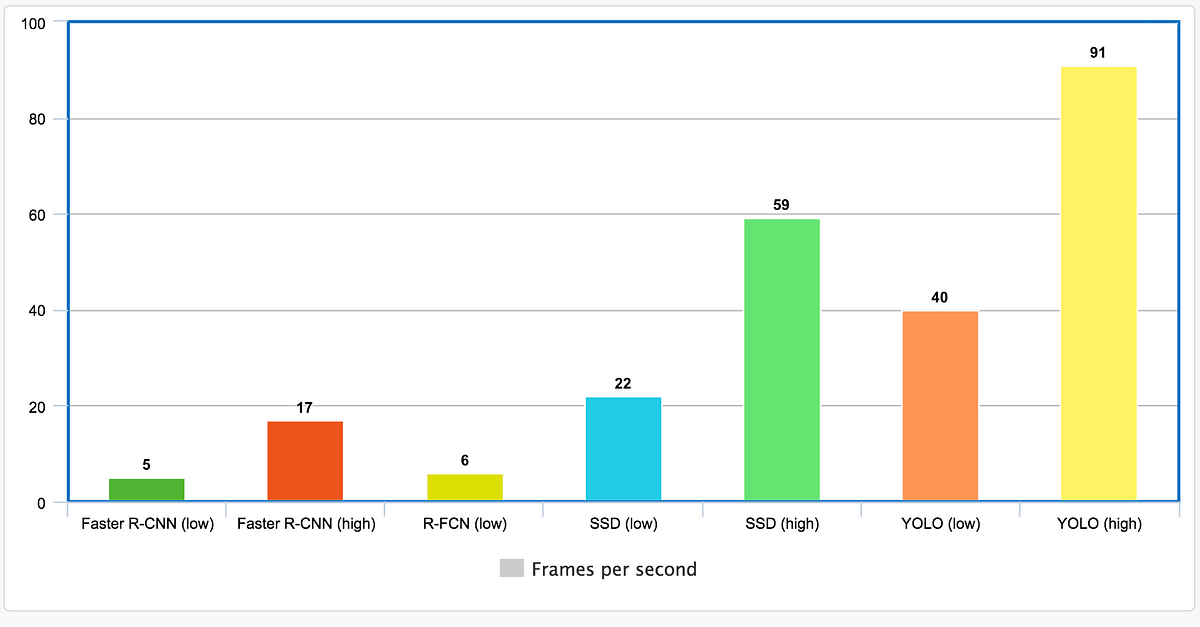
The Mean Average Precision is calculated by taking mean of the Average Precision values over different values of threshold, for example in the COCO Primary Challenge the mAP was calculated by averaging the AP scores over a range of IoU thresolds from 0.5 to 0.95 with a step size of 0.05 and finally taking the mean of the AP scores over all the classes. For more detailed explanation of mAP follow this blog - "Breaking Down Mean Average Precision". Now that we know how Object Detection Systems are evaluated let's checkout various methods for object detection. We'll compare various object detection model's performance against the MS COCO Dataset that contains 80 classes. We'll look at the Inference speed and mAP scores. Below is a plot showing the highest and lowest Frames Per Second (FPS) values reported in their respective papers.

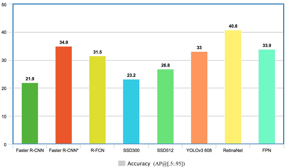
It is clear that YOLO object detection are faster by a huge margin compared to other object detection methods, however an important thing to note is the plot doesn't mention the mAP scorees for the models with the highest inference speeds. Now lets look at mAP scores for various methods against the MS COCO Dataset.

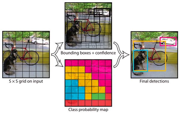
From the plot above we can see that RetinaNET has the highest mAP score of 40.8 followed by Faster-RCNN, FPN and YOLO. The difference between the latter three methods is not huge compared to their difference with RetinaNET which is SOTA in object detection. We can safely assume that YOLO will provide us with the right balance of Accuracy and Speed for our task of Fashion product detection and localisation. The research paper by Myntra used Mask RCNN for their object detection module since they had the luxury to run that part offline, however we do not have that luxury if we want to recommend similar products in real time using a web application. Hence we'll use YOLO object detection for detecting fashion products in three categories - topwear, bottomwear and footwear for our simplicity, we can easily improve our recommendation engine by including more and better categories for object detection like classifying the type of shirts, t-shirts, bags, sunglasses, trousers, jeans etc. YOLO refers to “You Only Look Once” is a versatile object detection model. YOLO algorithms divide a given input images into the SxS grid system. Each grid is responsible for object detection. Now the Grid cells predict the boundary boxes for the detected object. For every box, we have five main attributes: x and y for coordinates, w and h for width and height of the object, and a confidence score for that the box containing the object. Follow this blog for training an object detector using your custom dataset - "YOLOv5 Training for Custom Dataset"
Source: YOLO - You Only Look Once
Code snippet for training YOLOv5 model on custom dataset using Pytorch and Ultralytics Github repo.
!git clone https://github.com/ultralytics/yolov5
%cd yolov5
%pip install -qr requirements.txt

import torch
print('Setup complete. Using torch %s %s' % (torch.__version__, torch.cuda.get_device_properties(0) if torch.cuda.is_available() else 'CPU'))

!python train.py --img 640 --batch 2 --epochs 150 --data custom_dataset.yaml --weights /content/yolov5/weights/yolov5s.pt --nosave --cache
Your 'custom_dataset.yaml' file should look something like this
For training the custom Object Detection model we'll use Transfer Learning. We'll load YOLOv5s (s stands for small variant of YOLOv5) weights trained on the COCO Dataset and use transfer learning to fine-tune the model for our use case. I've created a dataset of 180 images (135 train and 45 validation) with annotated topwear, bottomwear and footwear. We were able to achieve a mAP score of 0.94 @ 0.5 IoU threshold on a test set of 45 images. Here are some object detection results on topwear, bottomwear and footwear detection.
Training summary for Topwear, Bottomwear and Footwear detection and localization
We use embedding generation to represent images/products such that similar ones are grouped together whereas dissimilar ones are moved away so that in order to retrieve products that are similar to the products present in the query image. There are various ways to calculate similarity between images after they are converted into a vector with n-dimensions. Cosine similarity and Euclidean distance are two examples. We can define Cosine similarity and Euclidean distance as -
In order to convert images to n-dimensional vector representations of the images, we'll use a special type of Neural Network called Siamese Network. It is network which takes in three inputs - anchor, positive and negative the inputs are such that anchor and positive inputs are similar whereas anchor and negative inputs are dissimilar. The output is three n-dimensional vectors representing anchor, positive and negative inputs generated by a CNN backbone. This network requires a special kind of loss function that minimizes the distance metric between anchor and positive while maximizing the distance metric between anchor and negative hence we'll need an intermediate layer that computes the distance between anchor and positve outputs and anchor and negative outputs. One such loss is the triplet loss which in our case we've defined as -
"Shop The Look" is a dataset taken from "Wang-Cheng Kang, Eric Kim, Jure Leskovec, Charles Rosenberg, Julian McAuley (2019). Complete the Look: Scene-based Complementary Product Recommendation". In Proceedings of IEEE Conference on Computer Vision and Pattern Recognition (CVPR'19). It provides the two datasets for fashion and home respectively with scene and product pairs. Product is an image of a product in professional setting whereas a scene is the image of the same product but in casual or non-professional setting. Each dataset contains the scene-product pairs in the following format, where scene and products are encoded with a signature that can be converted to an url by using a function provided in the official github repo STL-Dataset.
Example (fashion.json):
{
    "product": "0027e30879ce3d87f82f699f148bff7e",
    "scene": "cdab9160072dd1800038227960ff6467",
    "bbox": [
        0.434097,
        0.859363,
        0.560254,
        1.0
    ]
}
We can easily create anchor and positive pairs from this dataset and for generating negative samples we can randomly select scenes from the dataset which is not same as the positive sample.
We now move onto to define the Siamese network using Tensorflow and Keras. For a detailed explanation on the definition of the network, follow this tutorial from Keras
import tensorflow as tf
from tensorflow.keras.models import Model
from tensorflow.keras import losses, metrics, optimizers
from tensorflow.keras.applications import resnet
from tensorflow.keras.layers import Input, Flatten, Dense, BatchNormalization

TARGET_SHAPE = (224,224,3)
base_model = resnet.ResNet50(weights="imagenet", input_shape=TARGET_SHAPE, include_top=False)

for layer in base_model.layers:
    layer.trainable = True

x = Flatten()(base_model.output)
x = Dense(512, activation="relu")(x)
x = BatchNormalization()(x)
x = Dense(256, activation="relu")(x)
x = BatchNormalization()(x)

output = Dense(EMBEDDING_DIMENSION, activation="linear")(x)

embedding = Model(base_model.input, output, name="Embedding")

class DistanceLayer(tf.keras.layers.Layer):
    """
    This layer is responsible for computing the distance between the anchor
    embedding and the positive embedding, and the anchor embedding and the
    negative embedding.
    """

    def __init__(self, **kwargs):
        super().__init__(**kwargs)

    def call(self, anchor, positive, negative):
        ap_distance = tf.reduce_sum(tf.square(anchor - positive), -1)
        an_distance = tf.reduce_sum(tf.square(anchor - negative), -1)
        return (ap_distance, an_distance)

anchor_input = Input(name="anchor", shape=TARGET_SHAPE)
positive_input = Input(name="positive", shape=TARGET_SHAPE)
negative_input = Input(name="negative", shape=TARGET_SHAPE)

distances = DistanceLayer()(embedding(resnet.preprocess_input(anchor_input)), embedding(resnet.preprocess_input(positive_input)), embedding(resnet.preprocess_input(negative_input)))

siamese_network = Model(inputs=[anchor_input, positive_input, negative_input], outputs=distances)

class SiameseModel(Model):
    """The Siamese Network model with a custom training and testing loops.

    Computes the triplet loss using the three embeddings produced by the
    Siamese Network.

    The triplet loss is defined as:
       L(A, P, N) = max(‖f(A) - f(P)‖² - ‖f(A) - f(N)‖² + margin, 0)
    """

    def __init__(self, siamese_network, margin=0.5):
        super(SiameseModel, self).__init__()
        self.siamese_network = siamese_network
        self.margin = margin
        self.loss_tracker = metrics.Mean(name="loss")

    def call(self, inputs):
        return self.siamese_network(inputs)

    def train_step(self, data):
        with tf.GradientTape() as tape:
            loss = self._compute_loss(data)
        gradients = tape.gradient(loss, self.siamese_network.trainable_weights)
        self.optimizer.apply_gradients(zip(gradients, self.siamese_network.trainable_weights))
        self.loss_tracker.update_state(loss)
        return {"loss": self.loss_tracker.result()}

    def test_step(self, data):
        loss = self._compute_loss(data)
        self.loss_tracker.update_state(loss)
        return {"loss": self.loss_tracker.result()}

    def _compute_loss(self, data):
        ap_distance, an_distance = self.siamese_network(data)
        loss = ap_distance - an_distance
        loss = tf.maximum(loss + self.margin, 0.0)
        return loss

    @property
    def metrics(self):
        return [self.loss_tracker]

siamese_model = SiameseModel(siamese_network)
siamese_model.compile(optimizer=optimizers.Adam(1e-4))
Having trained the embeddingg generation model, we have to generate and save embeddings for the catalog of fashion products.
Having generated and stored the embeddings for the catalog of fashion products, the final step is to combine all the modules into a pipeline that takes in a query image and outputs the relevant recommendations. Before we startpredicting from our saved tensorflow models we can further optimize them by using a technique called post training quantization. Post-training quantization is a conversion technique that can reduce model size while also improving CPU and hardware accelerator latency, with little degradation in model accuracy. One can quantize an already-trained float TensorFlow model when its converted to TensorFlow Lite format using the TensorFlow Lite Converter. We will reduce the size of a floating point model by quantizing the weights to float16, it can virtually reduce the model size by half by converting all the float32 weights to float16. The below code snippet can be used to quantize Tensorflow-Keras models to Tensorflow-Lite models -
import tensorflow as tf
from tensorflow.keras.models import load_model()

# Path to your saved tensorflow-keras model
TFKERAS_MODEL_PATH = "model.h5"

# Path to save the tensorflow-lite model
TFLITE_MODEL_PATH = "model.tflite"
model = load_model(TFKERAS_MODEL_PATH)

tf_lite_converter = tf.lite.TFLiteConverter.from_keras_model(model)
tf_lite_converter.optimizations = [tf.lite.Optimize.OPTIMIZE_FOR_SIZE]
tf_lite_converter.target_spec.supported_types = [tf.float16]
tflite_model = tf_lite_converter.convert()

open(TFLITE_MODEL_PATH, "wb").write(tflite_model)
We can use the following code snippet to load and predict using a Tensorflow-Lite model.
import tensorflow as tf

class TFLiteModel:
    """
    Generic Class to load, initialize and predict using Tensorflow Lite Models
    """
    def __init__(self, model_path, batch_size, input_shape, output_shape):
        """
        Initialize interpretor, allocate input and output tensors
        """
        self.interpreter = tf.lite.Interpreter(model_path=model_path)
        self.input_details = self.interpreter.get_input_details()
        self.output_details = self.interpreter.get_output_details()
        self.interpreter.resize_tensor_input(self.input_details[0]['index'], (batch_size,) + input_shape)
        self.interpreter.resize_tensor_input(self.output_details[0]['index'], (batch_size,) +  output_shape)
        self.interpreter.allocate_tensors()
        self.input_details = self.interpreter.get_input_details()
        self.output_details = self.interpreter.get_output_details()

    def __call__(self, X):
        """
        Invoke the Tensorflow Lite model with the provided input and produce predictions/outputs
        """
        self.interpreter.set_tensor(self.input_details[0]['index'], X)
        self.interpreter.invoke()
        y = self.interpreter.get_tensor(self.output_details[0]['index'])
        return y

tflite_model = TFLiteModel(model_path=TFLITE_MODEL_PATH, batch_size=32, input_shape=(224,224,3), output_shape=(256,))
outputs = tflite_model(inputs)
Below are some plots showing the imporvements in the models after Post Training Quantization.
Quantization Summary for Gender Classification Model
Quantization Summary for Embedding Generation Model
After the models are optimized we can create the final pipeline as shown in the diagram below
Here are some example recommendations from the final pipeline. The first image is the query image followed by the recommendations
Query
Recommendation
Query
Recommendation
Query
Recommendation
Query
Recommendation
<iframe width="560" height="315" align="center" src=" https://www.youtube.com/embed/YlWKfkpZ9h0 " title="YouTube video player" frameborder="0" allow="accelerometer; autoplay; clipboard-write; encrypted-media; gyroscope; picture-in-picture" allowfullscreen></iframe>This system can be considered as a POC (Proof of Concept) for image similarity based item recommendation engine, further improvements can be made by changing the existing modules with better performing alternatives as the time progresses. For example we can switvh the object detection pipeline to any SOTA algorithms of the time for better detections. similarly we can retrain the embedding generation model regularly from time to time as new products are being added to the catalog. The current object detection only detects topwear, bottomwear and footwear we can imporve it by adding specific classes instead of broad terms, like shirts, t-shirts, suits, pants, trouser, jeans, shoes and also support for other fashion accessories like handbags, sunglasses, watches etc. The STL-Dataset included lot of pairs where the product and the scene did not match, we can clean the dataset of such pairs and retrain the embedding generation model for higher number of epochs. Lastly we need to deploy this system for users to try it out.
- Applied AI Course's Machine Learning Course
- Buy Me That Look: An Approach for Recommending Fashion Products
- Webscraping e-commerce websites using python
- Man/Woman classification dataset from Kaggle
- Breaking Down Mean Average Precision
- Object Detection Speed and Accuracy Comparision
- YOLOv5 Training for Custom Dataset
- YOLO - You Only Look Once
- Ultralytics YOLOv5
- Complete the Look: Scene-based Complementary Product Recommendation
- STL-Dataset
- Keras Tutorial for image similarity calculation


 Embeddings Learning


