-
Notifications
You must be signed in to change notification settings - Fork 82
BOSS 19 Tutorial
Welcome to the Cloudberry tutorial at BOSS 2019 co-located with VLDB 2019!
In this tutorial, you'll do the following steps:
-
Get your machine
- We provide each of you an AWS EC2 machine. You'll register your name to access one machine and keep its IP address for use.
-
Start Cloudberry and Twittermap
- Start your own Cloudberry middleware and Twittermap application on an AWS instance we provide.
- Test the Twittermap application to do visualization.
- Send example queries to Cloudberry RESTFul API
The following diagram illustrates the Twittermap architecture
Cloudberry BOSS 2019 AWS EC2 IPs
Important!
Suppose the IP address you registered is
ec2-35-163-10-157.us-west-2.compute.amazonaws.com,
let's call it [your aws ip].
ssh boss@[your aws ip]Type password: boss
If you see the following message, you're in! ^^
Last login: Wed Aug 21 17:31:55 2019 from dhcp-v097-215.mobile.uci.edu

       __|  __|_  )
       _|  (     /   Amazon Linux 2 AMI
      ___|\___|___|

https://aws.amazon.com/amazon-linux-2/
4 package(s) needed for security, out of 12 available
Run "sudo yum update" to apply all updates.
[boss@ip-172-31-29-92 ~]$ - 8GB memory
- 2 vCPUs
- OS: Amazon Linux
- Installed Software:
- Java 8 SDK
- sbt 0.13 (Scala building tool)
- AsterixDB
- Data:
- Sample tweets (1M): 2018-01-01 ~ 2019-08-24
Note Backend database (AsterixDB) is already installed and started. Web console of AsterixDB is at
http://[your aws ip]:19001
cd ~/cloudberry/cloudberrysbt "project neo" "run"Wait until you see the following messages:
[info] Loading project definition from /home/cloudberry/cloudberry/cloudberry/project
[info] Set current project to cloudberry (in build file:/home/cloudberry/cloudberry/cloudberry/)
[info] Set current project to neo (in build file:/home/cloudberry/cloudberry/cloudberry/)

--- (Running the application, auto-reloading is enabled) ---

[info] p.c.s.NettyServer - Listening for HTTP on /0:0:0:0:0:0:0:0:9000

(Server started, use Ctrl+D to stop and go back to the console...)ssh boss@[your aws ip]cd ~/cloudberry/examples/twittermapsbt "project web" "run 9001"Wait until the shell prints the following messages:
--- (Running the application, auto-reloading is enabled) ---

[info] p.c.s.NettyServer - Listening for HTTP on /0:0:0:0:0:0:0:0:9001

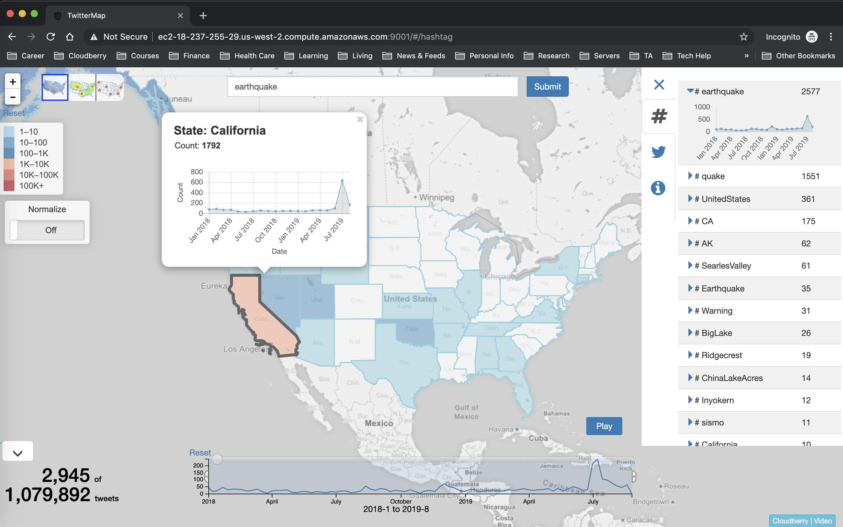
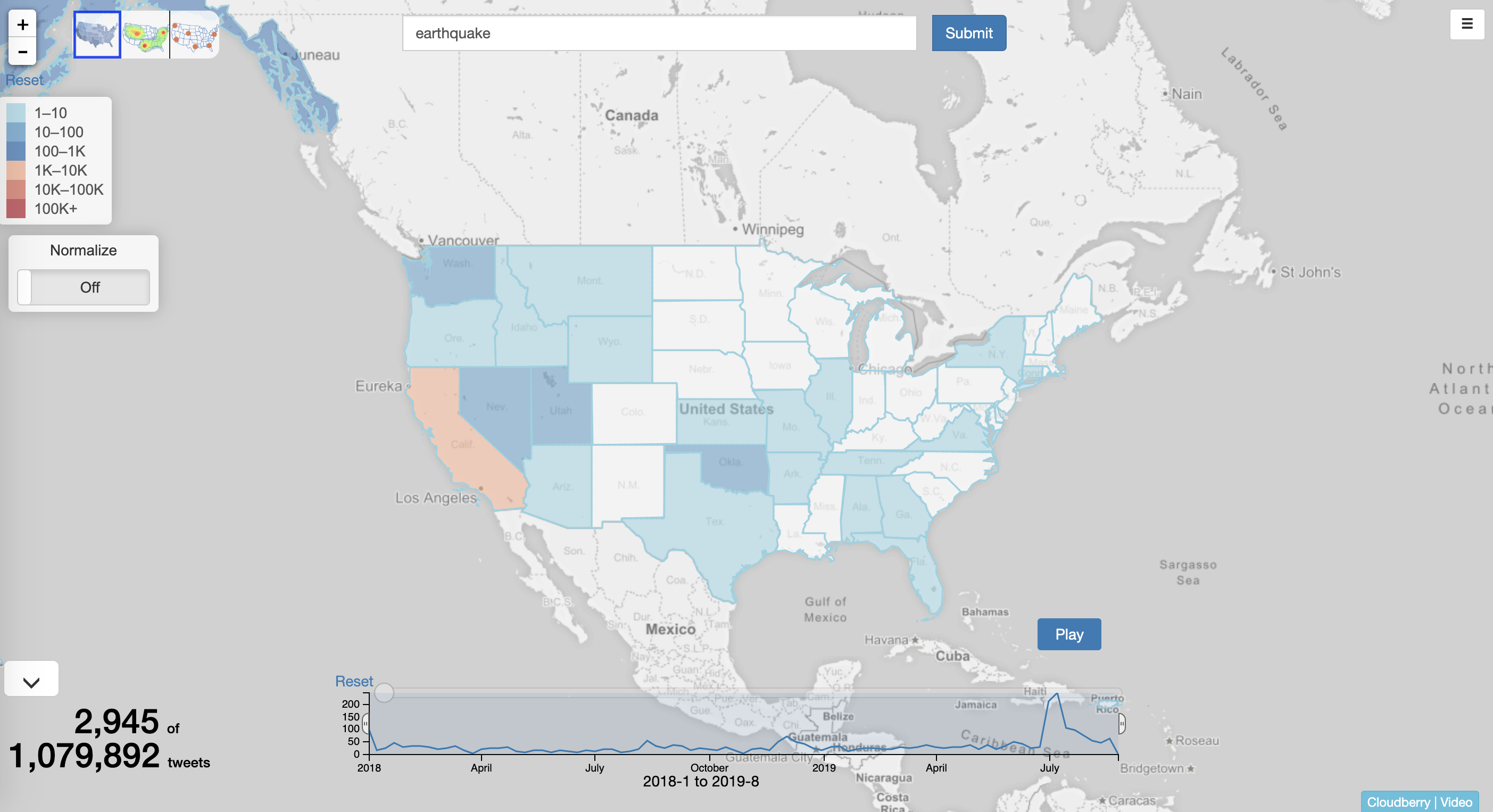
(Server started, use Ctrl+D to stop and go back to the console...)Use your Web browser to open the link http://[your aws ip]:9001. The first time you open the page, it could take up to several minutes to show the following Web page.
(Note: Firefox users need to go to about:config and change privacy.trackingprotection.enabled to false and restart Firefox.)
Congratulations! You have successfully set up TwitterMap using Cloudberry and AsterixDB!
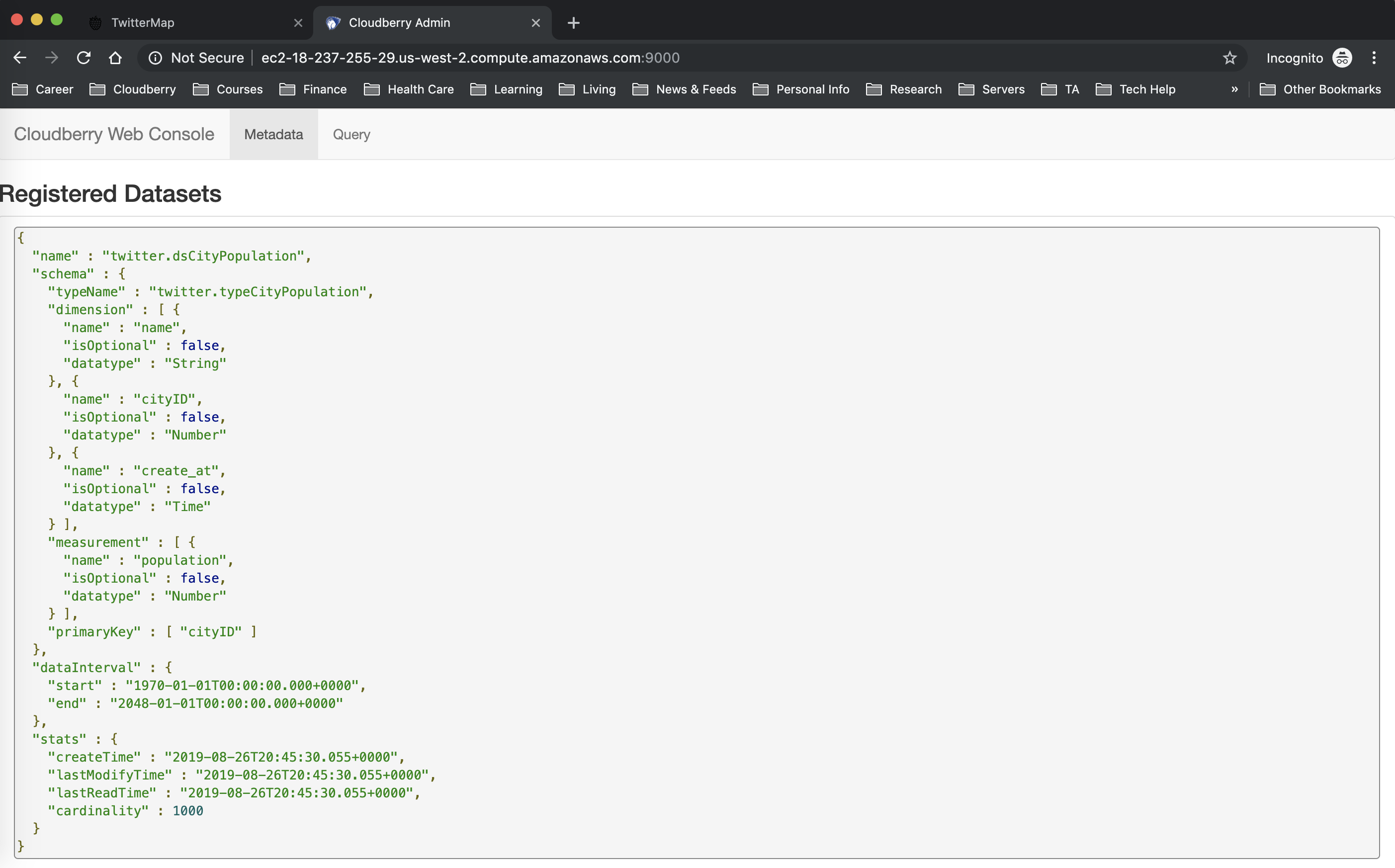
Access http://[your aws ip]:9000 to check the schema of the datasets in Cloudberry.
The below json object describes the schema used in the TwitterMap application, which is already registered in Cloudberry:
{
  "name":"twitter.ds_tweet",
  "schema":{
    ...
    "dimension":[
      {"name":"create_at","isOptional":false,"datatype":"Time"},
      {"name":"id","isOptional":false,"datatype":"Number"},
      {"name":"coordinate","isOptional":false,"datatype":"Point"},
      {"name":"hashtags","isOptional":true,"datatype":"Bag","innerType":"String"},
      {"name":"geo_tag.stateID","isOptional":false,"datatype":"Number"},
      {"name":"geo_tag.countyID","isOptional":false,"datatype":"Number"},
      {"name":"geo_tag.cityID","isOptional":false,"datatype":"Number"},
      ...
    ],
    "measurement":[
      {"name":"text","isOptional":false,"datatype":"Text"}
    ],
    ...
  },
  ...
}Access http://[your aws ip]:19001 to check the metadata table used by Cloudberry inside AsterixDB. Copy the following query to the Query box, and click the Run button.
select name as `viewName`, createQuery.`filter`[0] as `filter` from berry.meta where createQuery is not unknown;The result should include all the materialized views and their filtering conditions as follows.
{ "viewName": "twitter.ds_tweet_c5285abd05d46a954151ddf9b8128114", "filter": { "field": "text", "relation": "contains", "values": [ "hurricane" ] } }
...
Note: as we send more queries, more datasets (ds_tweet_[hash value]) are created as materialized views.
A request to the Cloudberry RESTful API is represented as a json object. You can use either the Web console or curl command to send such requests.
Access http://[your aws ip]:9000 -> query tab, copy a json request to the Query box, and click the Submit button.
cd ~/queries
curl -X POST -H "Content-Type: application/json" -d @[query filename] http://localhost:9000/berry
Type Ctrl+C to stop the query result mode from curl.
Return the tweet where the tweet ID is equal to a specific value
- Use case in Twittermap
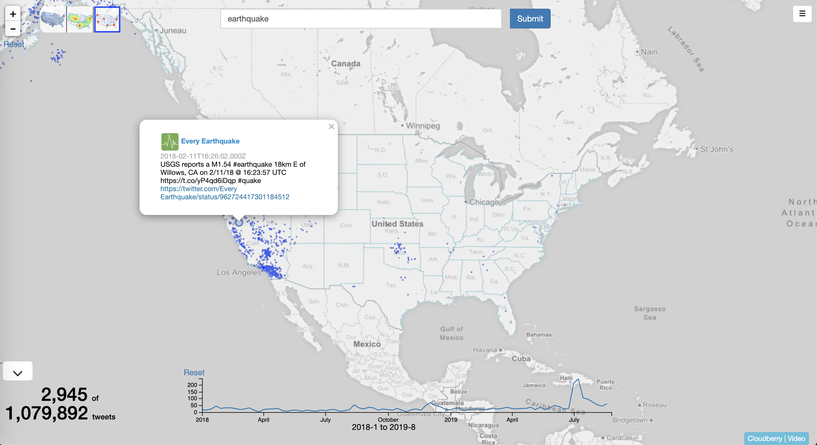
Hover over a tweet point on the scatterplot map:
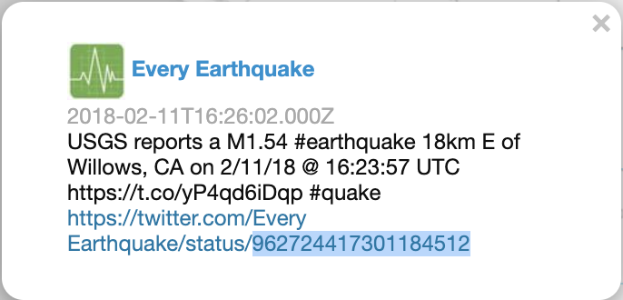
- Copy the
idvalue from the hyperlink and paste to thevaluesentry in the following query
{
  "dataset": "twitter.ds_tweet",
  "filter": [{
    "field": "id",
    "relation": "=",
    "values": "962724417301184512"
  }],
  "select" : {
    "order" : [],
    "limit": 1,
    "offset" : 0,
    "field": ["*"]
  }
}Return per-state count of tweets containing the keyword earthquake
Use Case in Twittermap: choropleth map
{
  "dataset": "twitter.ds_tweet",
  "filter": [
    {
      "field": "text",
      "relation": "contains",
      "values": ["earthquake"]
    }
  ],
  "group": {
    "by": [
        {
          "field": "geo_tag.stateID",
          "as": "state"
        }
      ],
    "aggregate": [
      {
        "field": "*",
        "apply": {
          "name": "count"
        },
        "as": "count"
      }
      ]
  }
}
Pay attention to the query time when there is no view. Now repeat Step 2, and see the newly added View. Repeat Step 3.2 and you will see the time is reduced due to the view.
Return per-day count of tweets containing the keyword earthquake
**Use case in Twittermap: Timebar **
{
  "dataset": "twitter.ds_tweet",
  "filter": [
    {
      "field": "text",
      "relation": "contains",
      "values": ["earthquake"]
    }
  ],
  "group": {
    "by": [
        {
          "field": "create_at",
          "apply": {
            "name": "interval",
            "args": {
              "unit": "day"
            }
          },
          "as": "day"
        }
      ],
    "aggregate": [
      {
        "field": "*",
        "apply": {
          "name": "count"
        },
        "as": "count"
      }
      ]
  }
}- Return per-state count of tweets containing the keyword
job.
{
  "dataset": "twitter.ds_tweet",
  "filter": [
    {
      "field": "text",
      "relation": "contains",
      "values": ["job"]
    }
  ],
  "group": {
    "by": [
        {
          "field": "geo_tag.stateID",
          "as": "state"
        }
      ],
    "aggregate": [
      {
        "field": "*",
        "apply": {
          "name": "count"
        },
        "as": "count"
      }
    ]
  }
}
If no materialized view is available for a popular keyword, the query could take a long time (10~15 seconds). We will next show how to address this long-latency issue.
Drum is a technique to support progressive results in batches. The following is an example query:
- Return per-state count of tweets containing the keyword
job. - Optionally return the results progressively with an interval of 500ms.
{
  "dataset": "twitter.ds_tweet",
  "filter": [
    {
      "field": "text",
      "relation": "contains",
      "values": ["job"]
    }
  ],
  "group": {
    "by": [
        {
          "field": "geo_tag.stateID",
          "as": "state"
        }
      ],
    "aggregate": [
      {
        "field": "*",
        "apply": {
          "name": "count"
        },
        "as": "count"
      }
    ]
  },
  "select" : {
    "order" : ["-count"],
    "limit": 100,
    "offset" : 0
  },
  "option":{
   "sliceMillis": 2000
  }
}
Notice how the results are returned in batches. Also notice the results of the last batch include the keyword "DONE" to indicate the full result returned. The response-time interval (called "rhythm") can be tuned in the SliceMillis option)
-
By default, Cloudberry returns the accumulated results progressively, i.e., the results returned in each batch are the entire aggregation numbers computed so far.
-
If you want the progressive results to only include those for each new batch, you can just add another entry into the
optionselement:returnDelta: true. -
Return per-state count of tweets containing the keyword
job -
Optionally return the results progressively with a time interval of 500ms in the
deltamode.
{
  "dataset": "twitter.ds_tweet",
  "filter": [
    {
      "field": "text",
      "relation": "contains",
      "values": ["job"]
    }
  ],
  "group": {
    "by": [
        {
          "field": "geo_tag.stateID",
          "as": "state"
        }
      ],
    "aggregate": [
      {
        "field": "*",
        "apply": {
          "name": "count"
        },
        "as": "count"
      }
    ]
  },
  "select" : {
    "order" : ["-count"],
    "limit": 100,
    "offset" : 0
  },
  "option":{
   "sliceMillis": 2000,
   "returnDelta": true
  }
}- Send the query again to see how the results are returned.
