Goal: A comparison study between different ML algorithms on forecasting flood events using open datasets from ECMWF/Copernicus.
Team: @lkugler, @seblehner
- Project description
- Dependencies and Setup
- Folder structure
- Data description
- Model structure
- ML techniques
- Acknowledgments
We plan to investigate various machine learning (ML) techniques for predicting floods. The main goal is a comparative study of some of the most promising ML methods on this proposed subject. As a side goal, the open source development approach via github will result in a nice basis for further work.
ERA5 data will be used as predictor to model either the probability of exceeding some threshold in river discharge by the GloFAS reanalysis or to predict the severeness of the event given by the ECMWF’s severe event catalogue. We plan to investigate the impact of different meteorological variables, starting with direct precipitation output and combinations of thermodynamic and dynamic variables. Additionally, the results can be compared with GloFAS forecast reruns as well. Thereby, the benefits and/or drawbacks of using ML techniques instead of coupled complex models can be explored.
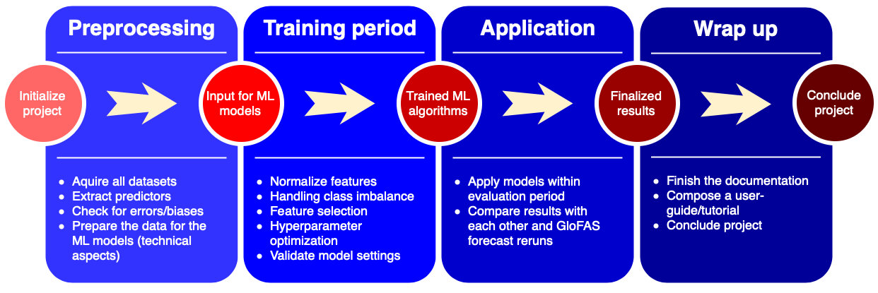
Our projected workflow can be seen below:
This repository was created for Python3 Dependencies can be found in the environment.yml file. Download the repository, move it to any path you wish for. You can either install all packages by hand, or you can use conda env create -f environment.yml for a one-step installation of all dependencies. When installed, a new environment named ml_flood is created. Remember to use
bash; conda activate ml_flood
before executing any script to ensure all packages exist.
To start jupyter in a specific conda environment, we had to activate the ipython kernel with
/path/to/home/.conda/envs/ml_flood/bin/python -m ipykernel install --user
before starting jupyter. Newer jupyter versions may allow you to switch environments from the menu bar inside jupyter.
To experiment with the notebooks, download the repository to your local device:
git clone https://github.com/esowc/ml_flood.gitA folder ml_flood has been created. It not only includes the notebooks but also a dataset for you to experiment around and develop your own extensions to existing models.
The folder structure will be as you would expect from the github webpage:
.
+-- data/
+-- notebooks/
|   +-- 1_data_download_analysis_visualization/
|   +-- 2_preprocessing/
|   +-- 3_model_tests/
|   +-- 4_coupled_model/
|   +-- resources/
+-- python/
|   +-- aux/
The data/ folder contains the small test dataset included in the repository. The notebooks folder contains all fully-reproducible notebooks that work with the small test dataset, except for the 4_coupled_model/ folder. The python/ folder contains work in progress scripts that were written in the process of creating this repo and may contain errors or be incomplete. The python/aux/ folder contains collections of code that is used throughout the notebooks.
We use ERA5 Reanalysis and GloFAS Reanalysis and forecast rerun data. A detailed description can be found in the notebook 1_data_download_analysis_visualization/1.03_data_overview.
For reproducibility, a small testing dataset is included in the folder ./data/ it allows you to execute all notebooks in the ./notebooks/ folder except for notebooks in ./notebooks/4_coupled_model/ which need data from a larger domain.
We implemented two major structures of ML models:
- The simpler, catchment based model which predicts the timeseries of discharge at a certain point given upstream precipitation etc. from ERA5.
- The more complex, regional coupled model
which predicts the next state (timestep) of river discharge from previous states (discharges) and water input (from the atmosphere). It is physics inspired and splits up the prediction of discharge at a certain point into
- water inflow from upstream river gridpoints and
- water inflow from subsurface flow and smaller rivers. The model is fitted for every river gridpoint separately, thus making the training process more complex than applying a single model to all gridpoints.
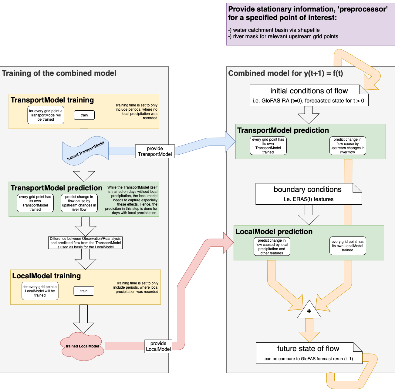
The model structure of the regional coupled model is layed out in the flowchart below. The model takes the influence of different features as well as their spatial and temporal state into account by spliting the whole process up into two models. The first encompasses changes in discharge happening due to non-local reasons (e.g. large-scale precipitation a few hundred kilometres upstream, affecting the flow at a certain point a few days later through river flow) and the second includes local effects from features like precipitation/runoff and their impact on discharge by subsurface flow or smaller rivers. For more detail see the notebooks in the /notebooks/ folder.
The techniques include:
- LinearRegression via sklearn
- SupportVectorRegressor via sklearn
- GradientBoostingRegressor via sklearn
- (Time-delayed) Neural Net via keras
We acknowledge the support of ECMWF and Copernicus for bringing this project to life!

