Adapting the PLE Settings

Adapting the PLE Settings

Parameter uncertainty analyses in d2d are mainly handled by exploiting the Profile Likelihood, which is initialized by calling the function arPLEInit which sets up the struct ar.ple containing the default specifications for the Profile Likelihood Algorithm. Subsequently, parameter profiles are calculated by use of the function ple, sampling the profile likelihood by iteratively proposing parameter steps and locally optimizing the objective function with the profile parameter being constrained. Since the default settings may not always work satisfactorily, this article summarizes the most important algorithm configurations which can be easily modified by the user and some useful functions related to this problem. To this end, a short introduction to how ple actually proposes parameter steps is necessary.

Profile Likelihood Sampling

It is usually just required that the likelihood profile crosses a certain objective function threshold if possible, thus these profiles need only to be calculated up until this point. Since it is not previously known for which parameters this threshold is crossed, profiles need to be calculated iteratively, sampling the profile towards the lower and upper parameter threshold by repetition of

1. Start from $P_{Last} = P_{New}$
2. Propose a parameter step $P_{Trial} = P_{Last} + P_{Step}$
3. Constrained Fit to new optimum: $P_{New} \gets P_{Trial}$

where $P_{Step}$ is necessarily required to change the profile parameter in each iteration.

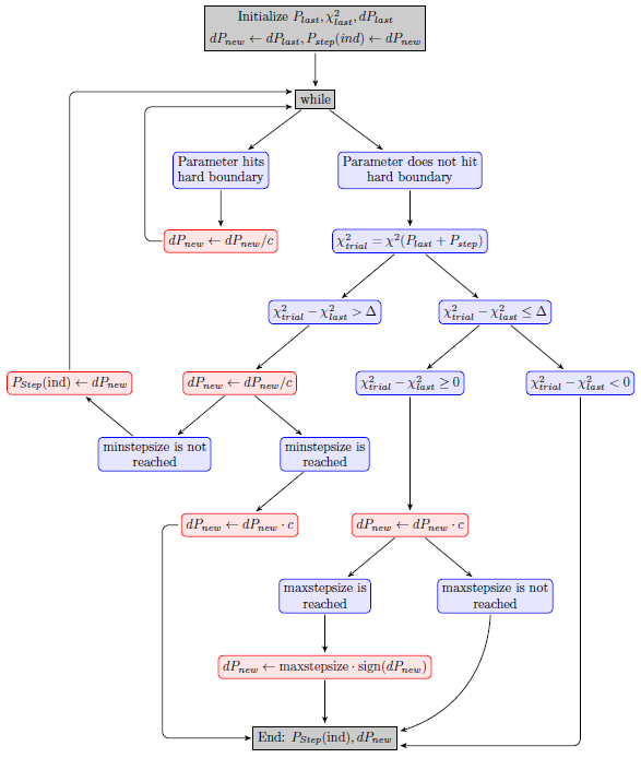
For such an iterative method to be applicable over a broad range of problems, the step choice needs to adapt to many possible forms of the profile. Since the objective function threshold is unchanged over all possible cases, the step size adaption should be related to the changes in the objective function values. This is implemented by adapting the step size until the criterion

$$ \chi^2(P_{Trial}) - \chi^2(P_{Last}) \le \Delta$$

is met. Since $\chi^2(P_{Trial})$ certainly decreases after fitting, $\Delta$ acts as an upper limit for the observed change of the objective function after reoptimization.

Direct Step Choice

In the current implementation, the default step choice algorithm proposes steps only in the profile parameter, leaving all other parameters unchanged.

$dP_{new}$ becomes the dP_{last} for the next iteration, determining which parameter step is used as a first trial.

Inert Step Choice

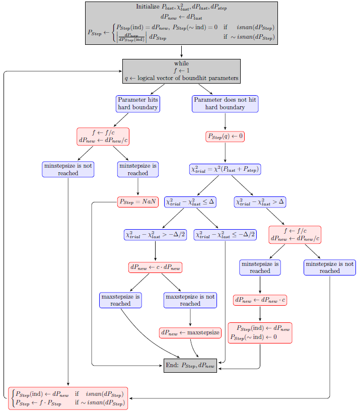
From theoretical considerations it seems promising to use prior information on the trajectory of the profile through parameter space to propose the next step. Such an alternative step choice is implemented simply by using the direction of the previously made step.

The fact that this flowchart looks more involved than the last one is due to stability issues arising from changing many parameters at once in each step. Hence, although in theory such a step choice is simple, the implementation gets messy and this is bound to happen to any other algorithm proposing steps in various directions.

Changing algorithm properties

Understanding the basic principle of these methods allows us to understand and modify various settings of the profile likelihood algorithm. Note that most options have to be set after arPLEInit is called, since the defaults are set by this function.

• Changing the step choice algorithm is done by setting the argument mode in arPLEInit([],[],mode). mode = 1 corresponds to the direct step choice (default), while mode = 2 switches to the inert choice. Extensive testing of the inert step choice in comparison to the direct choice revealed a massive increase in performance as measured by timing and whether the profiles actually reach the threshold if possible. This is a result of the proposed steps changing the objective function in a manner which is closer to the upper limit in most cases, making sampling only as dense as it needs to be. However in a tiny subset of cases, the inert step choice may behave less stably than the direct step choice in models with poorly specified integration or fit tolerances or for profiles with too many peaks. Nevertheless, use of mode = 2 is encouraged and if it proves its worth over time, this should be used as a new default.

• Default maximal and minimal stepsizes are stored in ar.ple.maxstepsize and ar.ple.minstepsize . While the maximal stepsize is proportional to the range of the parameter space of the profile parameter, the minimal stepsize is a default constant. Thus, changing the minstepsize might be necessary for some parameters, while the maximal stepsize is usually roughly satisfactory. Note that these stepsizes exclusively correspond to the size of the step in the profile parameter.

• ar.ple.samplesize specifies the maximal number of steps attempted in the negative and positive direction from the starting point and is set to 100 by default. If the algorithm terminates prematurely because of this condition, the function pleExtend can be used to recover without recalculation of the whole profile.

• The upper limit $\Delta$ is set in ar.ple.relchi2stepincrease as a relative factor (0.1) with respect to the profile threshold icdf('chi2',0.95,1)$\approx 3.84$ (which in theory is used to construct 95%-confidence intervals) and this can be modified to influence sampling sparsity. Note that increasing this factor might empirically make the sampling density more appropriate, but it makes the algorithm more prone to errors since the theoretical upper limit for each step is increased simultaneously.

• While searching for the optimal step size, the proposed step $P_{Step}$ is varied by ar.ple.stepfaktor (default = 1.5) and the objective function needs to be re-evaluated for the new $P_{Trial}$. Looking for a step factor value which maximizes performance in a general setting may be worthwile, although not relevant for the day-to-day user.

Other notable options

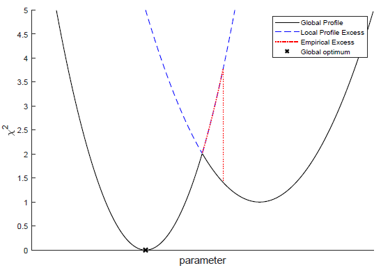
• Due to optimization after each step being local, the existance of local optima may lead to peaks or jumps in the sampled profile, although a profile should always be continuous by definition. This can be fixed by use of the function pleSmooth, which smoothens these peaks to the true profile form.

• In order to recover plots for individual profiles after they have already been calculated, use the function plePlot.

• To suppress the plotting which happens in parallel to the profile sampling, set the flag ar.ple.showCalculation = 0 . Especially for less time intensive models the relative difference in run time is appreciable.

• In order to get a feeling of how parameter changes along the profile influence predicted model trajectories, use arPLETrajectories.

• By setting the flag ar.ple.allowbetteroptimum = 1 the profile calculation sets a new optimum if an optimum with smaller objective function value is found while scanning the parameter space by virtue of the profile calculation. In this context, setting the new optimum means that the corresponding parameters ar stored in ar.p and automatically used as the initials for the following profiles. Caution: A new optimum is only recognized if decreases the objective function by ar.ple.optimset_tol, which takes the value 0.1 by default.

• By default, integration of the model trajectories in the ple-setting is performed without relying on sensitivities to decrease computational effort. This works reasonable enough in most instances, although it can be a severe source of problems in models with complicated objective function landscapes. Switching to ar.ple.usesensis = true forces the integrator to use sensitivites, yielding more accurate predictions. Hint: If ar.ple.chi2sinit - ar.ple.chi2s < 0 for any value of the index, this is a good indicator that integration might be problematic, since in theory this is prohibited.

• For a pool of various reasons, it might not be desirable to specify a saving directory every time arPLEInit is called. By setting the fourth argument in this function to false, automatic saving is turned off. In default settings, the progress is saved after calculation of a profile is finished.